Josh De La Rosa wanted to know how to do quadratic trend tests such as these in the R survey package 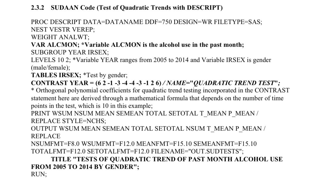
If you can’t read the image, the code extracts a sets of means for years from 2005 to 2014 and then tests a particular linear contrast of them, with coefficients c(6, 2, -1, -3, -4, -4, -3, -1, 2, 6)
I thought this would be easy: just do a linear model with a quadratic in year, and test the quadratic term. Unfortunately, the code example doesn’t give the output. And there isn’t a 2005 to 2014 combined file available. But there is a 2002-14 combined file. It’s huge, but I read it in and saved a subset.
load("~/nsduh_subset.rda")
library(survey)
## Loading required package: grid## Loading required package: Matrix## Loading required package: survival##
## Attaching package: 'survey'## The following object is masked from 'package:graphics':
##
## dotchartdes<-svydesign(id=~verep, strata=~vestr,nest=TRUE,
weight=~ANALWC10, data=nsduh)
des## Stratified 1 - level Cluster Sampling design (with replacement)
## With (220) clusters.
## svydesign(id = ~verep, strata = ~vestr, nest = TRUE, weight = ~ANALWC10,
## data = nsduh)cc<-c(6, 2, -1, -3, -4, -4, -3, -1, 2, 6)After I get around to the necessary rewrite, it will be possible to just use svyby and svymean to get the means of alcmon for each year and svycontrast to compute the contrast. At the moment, that way only works if you have a replicate-weight design. And it’s a bit slow, because there are 220 sets of replicate weights.
nsduh_jk<-as.svrepdesign(des,type="JKn")
jkmns<-svyby(~alcmon,~year, svymean, na.rm=TRUE,
             design=nsduh_jk, covmat=TRUE)
jkmns
## year alcmon se
## 2005 2005 0.5167334 0.003912681
## 2006 2006 0.5079644 0.003980633
## 2007 2007 0.5100226 0.004195848
## 2008 2008 0.5160143 0.004883058
## 2009 2009 0.5213838 0.004251909
## 2010 2010 0.5173512 0.003350081
## 2011 2011 0.5139415 0.004566130
## 2012 2012 0.5205190 0.004227852
## 2013 2013 0.5189917 0.004902192
## 2014 2014 0.5277706 0.003236195svycontrast(jkmns,cc)## contrast SE
## contrast 0.045587 0.0439We could use a single call to svymean, and then compute the proportions from it. I’m doing this to show it’s possible, not because you should do it this way. The point estimate is identical to the previous version; the standard error is equal at least to three figures (it could be different because it’s from Horvitz-Thompson estimator, not the jackknife).
des<-update(des, alcyr=interaction(alcmon,year))
mns <- svymean(~alcyr,na.rm=TRUE,design=des)
mns
## mean SE
## alcyr0.2005 0.046321 5e-04
## alcyr1.2005 0.049529 7e-04
## alcyr0.2006 0.047705 5e-04
## alcyr1.2006 0.049249 5e-04
## alcyr0.2007 0.047857 6e-04
## alcyr1.2007 0.049815 6e-04
## alcyr0.2008 0.047648 7e-04
## alcyr1.2008 0.050801 7e-04
## alcyr0.2009 0.047497 6e-04
## alcyr1.2009 0.051741 7e-04
## alcyr0.2010 0.048240 6e-04
## alcyr1.2010 0.051708 6e-04
## alcyr0.2011 0.049343 7e-04
## alcyr1.2011 0.052174 6e-04
## alcyr0.2012 0.049140 5e-04
## alcyr1.2012 0.053346 7e-04
## alcyr0.2013 0.049739 6e-04
## alcyr1.2013 0.053666 8e-04
## alcyr0.2014 0.049339 5e-04
## alcyr1.2014 0.055142 6e-04ratios<-svycontrast(mns,
list(alc05=quote(alcyr1.2005/(alcyr0.2005+alcyr1.2005)),
alc06=quote(alcyr1.2006/(alcyr0.2006+alcyr1.2006)),
alc07=quote(alcyr1.2007/(alcyr0.2007+alcyr1.2007)),
alc08=quote(alcyr1.2008/(alcyr0.2008+alcyr1.2008)),
alc09=quote(alcyr1.2009/(alcyr0.2009+alcyr1.2009)),
alc10=quote(alcyr1.2010/(alcyr0.2010+alcyr1.2010)),
alc11=quote(alcyr1.2011/(alcyr0.2011+alcyr1.2011)),
alc12=quote(alcyr1.2012/(alcyr0.2012+alcyr1.2012)),
alc13=quote(alcyr1.2013/(alcyr0.2013+alcyr1.2013)),
alc14=quote(alcyr1.2014/(alcyr0.2014+alcyr1.2014))
))
ratios## nlcon SE
## alc05 0.51673 0.0039
## alc06 0.50796 0.0040
## alc07 0.51002 0.0042
## alc08 0.51601 0.0049
## alc09 0.52138 0.0043
## alc10 0.51735 0.0034
## alc11 0.51394 0.0046
## alc12 0.52052 0.0042
## alc13 0.51899 0.0049
## alc14 0.52777 0.0032svycontrast(ratios, cc)## contrast SE
## contrast 0.045587 0.0439Using svymean like this isn’t necessary, because as statisticians we already have a tool for computing means and contrasts of means: regression. The domain mean by subsetting is exactly the same as the domain computed by regression (this is how I first understood domain estimation in surveys and the standard error estimation issues). We want an indicator variable for each year, and no intercept.
model0<-svyglm(alcmon~0+year,design=des)
model0
## Stratified 1 - level Cluster Sampling design (with replacement)
## With (220) clusters.
## update(des, alcyr = interaction(alcmon, year))
##
## Call: svyglm(formula = alcmon ~ 0 + year, design = des)
##
## Coefficients:
## year2005 year2006 year2007 year2008 year2009 year2010 year2011 year2012
## 0.5167 0.5080 0.5100 0.5160 0.5214 0.5174 0.5139 0.5205
## year2013 year2014
## 0.5190 0.5278
##
## Degrees of Freedom: 557742 Total (i.e. Null); 101 Residual
## Null Deviance: 288400
## Residual Deviance: 139300 AIC: 1267000svycontrast(model0, cc)## contrast SE
## contrast 0.045587 0.0439But there should be an even simpler way. Quadratic trend tests computed post hoc are what you do before you invent regression models. Surely we can just fit a model with linear and quadratic terms and test the quadratic term?
des<-update(des,numyr=as.numeric(year))
model2<-svyglm(alcmon~poly(numyr,2), design=des)
summary(model2)
##
## Call:
## svyglm(formula = alcmon ~ poly(numyr, 2), design = des)
##
## Survey design:
## update(des, numyr = as.numeric(year))
##
## Coefficients:
## Estimate Std. Error t value Pr(>|t|)
## (Intercept) 0.517067 0.001453 355.814 < 2e-16 ***
## poly(numyr, 2)1 2.831108 0.955914 2.962 0.00376 **
## poly(numyr, 2)2 0.943930 0.906141 1.042 0.29988
## ---
## Signif. codes: 0 '***' 0.001 '**' 0.01 '*' 0.05 '.' 0.1 ' ' 1
##
## (Dispersion parameter for gaussian family taken to be 0.2496892)
##
## Number of Fisher Scoring iterations: 2The numerical value is different because of different scaling, but the ratio of coefficient to standard error should be the same
coef(svycontrast(model0, cc))/SE(svycontrast(model0, cc))## contrast
## contrast 1.038224coef(model2)[3]/SE(model2)[3]## poly(numyr, 2)2
## 1.041703Only not.
The difference didn’t depend (as it shouldn’t) on how I parametrised the quadratic in model2: centering, scaling, even transforming to use exactly the c(6, 2, -1, -3, -4, -4, -3, -1, 2, 6) coefficients from SUDAAN.
After some considerable time, I realised the corresponding linear model was much uglier
des<-update(des,oyear=ordered(year))
omodel<-svyglm(alcmon~oyear, design=des)
summary(omodel)
##
## Call:
## svyglm(formula = alcmon ~ oyear, design = des)
##
## Survey design:
## update(des, oyear = ordered(year))
##
## Coefficients:
## Estimate Std. Error t value Pr(>|t|)
## (Intercept) 0.5170693 0.0014517 356.176 < 2e-16 ***
## oyear.L 0.0120422 0.0040586 2.967 0.00375 **
## oyear.Q 0.0039679 0.0038218 1.038 0.30165
## oyear.C 0.0005879 0.0040143 0.146 0.88386
## oyear^4 0.0088994 0.0039333 2.263 0.02580 *
## oyear^5 -0.0044635 0.0050910 -0.877 0.38270
## oyear^6 0.0004774 0.0037700 0.127 0.89948
## oyear^7 0.0046641 0.0040921 1.140 0.25707
## oyear^8 0.0031820 0.0040965 0.777 0.43911
## oyear^9 -0.0002011 0.0042115 -0.048 0.96202
## ---
## Signif. codes: 0 '***' 0.001 '**' 0.01 '*' 0.05 '.' 0.1 ' ' 1
##
## (Dispersion parameter for gaussian family taken to be 0.2496762)
##
## Number of Fisher Scoring iterations: 2coef(omodel)[3]/SE(omodel)[3]## oyear.Q
## 1.038224The linear model corresponding to the trend test has a complete set of orthogonal polynomials, and you look at the quadratic term.
So, now we have multiple ways to get the same answer in R as in SUDAAN, but I think looking at the regression models gives a fairly strong argument not to do that and to fit a much more straightforward regression model.