Multiple-response data is like factor data, except that you can be in more than one category. Examples include
- what is your ethnicity? (or, in the US, race/ethnicity, sigh)
- what social media do you use?
- what countries have you been to?
- what birds did you see this week?
I have the first version of a package to manipulate this sort of data, called rimu. The name stands for responses in multiplex, but rimu is also the name of a New Zealand tree, Dacrydium cupressinum, an attractive conifer with reddish wood.
Comments on the package and whether there are useful things it doesn’t do would be welcome. So far I have not considered modelling multiple-response data, nor the use of survey weights. If people are interested, I might do those in the future.
Here are selections from the two package vignettes.
Ethnicity
The usethnicity data set contains variables on race and ethnic identification from the 2017 Youth Risk Behaviour Survey, together with two variables on smoking behaviour. The YRBS is a multistage cluster-sampled survey, so valid inference about associations requires using survey design information. This subset of variables without weights is useful only for demonstration purposes.
library(rimu)## Loading required package: ggplot2data(usethnicity)
head(usethnicity)## Q4 Q5 QN30 QN31
## 1 2 E 2 2
## 2 1 2 2
## 3 1 A 1 2
## 4 1 2 2
## 5 2 E 2 2
## 6 2 E 1 1Question 4 asks Are you Hispanic or Latino?, and Question 5 asks for any of
- A. American Indian or Alaska Native,
- B. Asian,
- C. Black or African American,
- D. Native Hawaiian or Other Pacific Islander,
- E. White
that apply. In the data set, these five letters are pasted together into a single variable.
We need to split Q5 into its component letters. One way is to use strsplit, producing a list with a vector of zero to five letters for each individual, then call the as.mr method for lists.
race<-as.mr(strsplit(as.character(usethnicity$Q5),""))
mtable(race)
## E A C B D H F G
## 8306 863 3643 1014 847 455 7 5 1There’s a spurious " " category from the string splitting, and the values F, G, and H are also invalid, so we need to remove them
race<-mr_drop(race,c(" ","F","G","H"))
mtable(race)
## E A C B D
## 8306 863 3643 1014 455We might want easier-to-recognise names for the categories
race <- mr_recode(race, AmIndian="A",Asian="B", Black="C", Pacific="D", White="E")Now, Hispanic/Latino ethnicity is asked in a separate question. We convert it via the as.mr method for logical vectors, and then combine it with race
hispanic<-as.mr(usethnicity$Q4==1, "Hispanic")
ethnicity<-mr_union(race, hispanic)
ethnicity[101:120]
## [1] "Black" "Black" "Black"
## [4] "Black" "AmIndian+Black" "Black"
## [7] "Black" "Black" "Black"
## [10] "Black" "Black" "Black"
## [13] "Black+?Hispanic" "Black" "Black"
## [16] "Black" "Black" "Black"
## [19] "White+AmIndian+Black" "Black"The plot method shows co-occurence of the various race/ethnicity terms
plot(ethnicity,nsets=6)## Warning: Removed 1 rows containing missing values (geom_bar).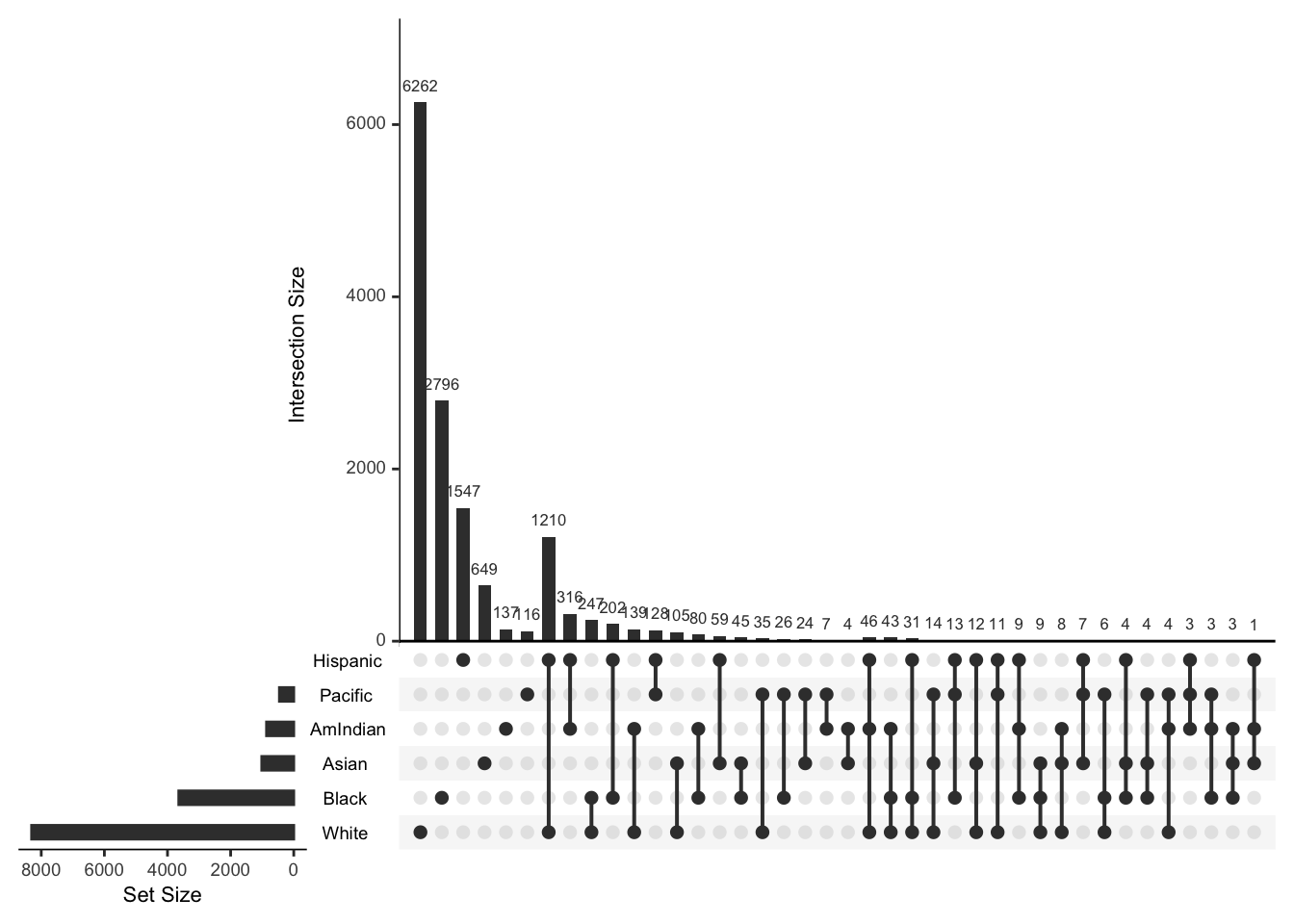
Tabulations against other factor or multiple-response variables are possible with mtable. Note that mtable shows frequencies for each category; use as.character to get frequencies for combinations – do not use as.factor, which is not generic and so cannot have a mr method.
mtable(ethnicity, usethnicity$QN30)## 2 1 <NA>
## White 4759 2112 0
## AmIndian 466 242 0
## Black 2000 612 0
## Asian 679 154 0
## Pacific 256 120 0
## Hispanic 2301 889 0table(ethnicity %has% "Black", usethnicity$QN30)##
## 1 2
## FALSE 2704 6596
## TRUE 612 2000table(ethnicity %hasonly% "Black", usethnicity$QN30)##
## 1 2
## FALSE 2878 7015
## TRUE 438 1581table(as.character(ethnicity), usethnicity$QN30)##
## 1 2
## 27 106
## AmIndian 40 65
## AmIndian+Asian 0 1
## AmIndian+Asian+Hispanic 0 1
## AmIndian+Asian+Pacific+Hispanic 1 0
## AmIndian+Black 11 48
## AmIndian+Black+Asian 1 2
## AmIndian+Black+Asian+Pacific 0 0
## AmIndian+Black+Asian+Pacific+Hispanic 0 1
## AmIndian+Black+Hispanic 3 5
## AmIndian+Black+Pacific 0 2
## AmIndian+Black+Pacific+Hispanic 0 1
## AmIndian+Hispanic 84 188
## AmIndian+Pacific 2 3
## AmIndian+Pacific+Hispanic 0 3
## Asian 80 489
## Asian+Hispanic 14 25
## Asian+Pacific 8 15
## Asian+Pacific+Hispanic 3 2
## Black 438 1581
## Black+Asian 2 26
## Black+Asian+Hispanic 1 0
## Black+Asian+Pacific 1 2
## Black+Asian+Pacific+Hispanic 0 1
## Black+Hispanic 40 100
## Black+Pacific 2 14
## Black+Pacific+Hispanic 6 6
## Hispanic 375 1010
## Pacific 31 72
## Pacific+Hispanic 34 68
## White 1618 3510
## White+AmIndian 50 71
## White+AmIndian+Asian 1 5
## White+AmIndian+Asian+Hispanic 0 1
## White+AmIndian+Asian+Pacific 0 1
## White+AmIndian+Black 13 20
## White+AmIndian+Black+Asian 2 2
## White+AmIndian+Black+Asian+Hispanic 1 1
## White+AmIndian+Black+Asian+Pacific 3 3
## White+AmIndian+Black+Asian+Pacific+Hispanic 2 6
## White+AmIndian+Black+Hispanic 5 7
## White+AmIndian+Black+Pacific 1 0
## White+AmIndian+Black+Pacific+Hispanic 1 3
## White+AmIndian+Hispanic 20 21
## White+AmIndian+Pacific 1 3
## White+AmIndian+Pacific+Hispanic 0 2
## White+Asian 19 71
## White+Asian+Hispanic 2 8
## White+Asian+Pacific 5 9
## White+Asian+Pacific+Hispanic 3 2
## White+Black 59 140
## White+Black+Asian 3 4
## White+Black+Asian+Hispanic 2 1
## White+Black+Asian+Pacific 0 0
## White+Black+Hispanic 11 19
## White+Black+Pacific 1 4
## White+Black+Pacific+Hispanic 3 1
## White+Hispanic 274 812
## White+Pacific 8 26
## White+Pacific+Hispanic 4 6table(forcats::fct_lump(as.character(ethnicity), n=10), usethnicity$QN30)##
## 1 2
## 27 106
## AmIndian 40 65
## AmIndian+Hispanic 84 188
## Asian 80 489
## Black 438 1581
## Black+Hispanic 40 100
## Hispanic 375 1010
## White 1618 3510
## White+Black 59 140
## White+Hispanic 274 812
## Other 281 595Birds
The birds dataset is a small subset of data from the Great Backyard Bird Count, in the US and Canada. We have counts of 12 birds by US county and Canadian province. The twelve birds are
library(rimu)
data(birds)
names(birds)[1:12]
## [1] "Phalaenoptilus nuttallii" "Fregata magnificens"
## [3] "Melanerpes lewis" "Melospiza georgiana"
## [5] "Rallus limicola" "Myioborus pictus"
## [7] "Poecile gambeli" "Aythya collaris"
## [9] "Xanthocephalus xanthocephalus" "Gracula religiosa"
## [11] "Icterus parisorum" "Coccyzus erythropthalmus"There’s a thirteenth column giving the location name.
These birds are perhaps more familiar as
- Common poorwill, Phalaenoptilus nuttallii
- Frigatebird Fregata magnificens
- Lewis’s woodpecker Melanerpes lewis
- Swamp sparrow Melospiza georgiana
- Virginia rail Rallus limicola
- Painted redstart Myioborus pictus
- Mountain chickadee Poecile gambeli
- Ring-necked duck Aythya collaris
- Yellowheaded blackbird Xanthocephalus xanthocephalus
- Common hill myna Gracula religiosa
- Scott’s oriole Icterus parisorum
- Black-billed cuckoo Coccyzus erythropthalmus
First, let’s put them into the data structures
bird_count <- as.ms(birds[,-13],na.rm=TRUE)
bird_presence <- as.mr(bird_count)
The bird counts will print like a sparse matrix
head(bird_count)## Phalaenoptilus nuttallii Fregata magnificens Melanerpes lewis
## [1,] . . .
## [2,] . . .
## [3,] . . .
## [4,] . . .
## [5,] . . .
## [6,] . . .
## Melospiza georgiana Rallus limicola Myioborus pictus Poecile gambeli
## [1,] . . . .
## [2,] . . . .
## [3,] 5 . . .
## [4,] . . . 30
## [5,] . . . .
## [6,] 1 . . .
## Aythya collaris Xanthocephalus xanthocephalus Gracula religiosa
## [1,] . . .
## [2,] 1 . .
## [3,] 4 . .
## [4,] 10 . .
## [5,] . . .
## [6,] 1 . .
## Icterus parisorum Coccyzus erythropthalmus
## [1,] . .
## [2,] . .
## [3,] . .
## [4,] . .
## [5,] . .
## [6,] . .but the bird presence/absence data has a more compact character form
head(bird_presence)## [1] ""
## [2] "Aythya collaris"
## [3] "Melospiza georgiana+Aythya collaris"
## [4] "Poecile gambeli+Aythya collaris"
## [5] ""
## [6] "Melospiza georgiana+Aythya collaris"What birds are most often present?
mtable(bird_presence)## Phalaenoptilus nuttallii Fregata magnificens Melanerpes lewis
## 9 16 87
## Melospiza georgiana Rallus limicola Myioborus pictus Poecile gambeli
## 876 121 4 317
## Aythya collaris Xanthocephalus xanthocephalus Gracula religiosa
## 1090 80 1
## Icterus parisorum Coccyzus erythropthalmus
## 8 1And what birds tend to go together? We can draw an upset chart
plot(bird_presence,nsets=12)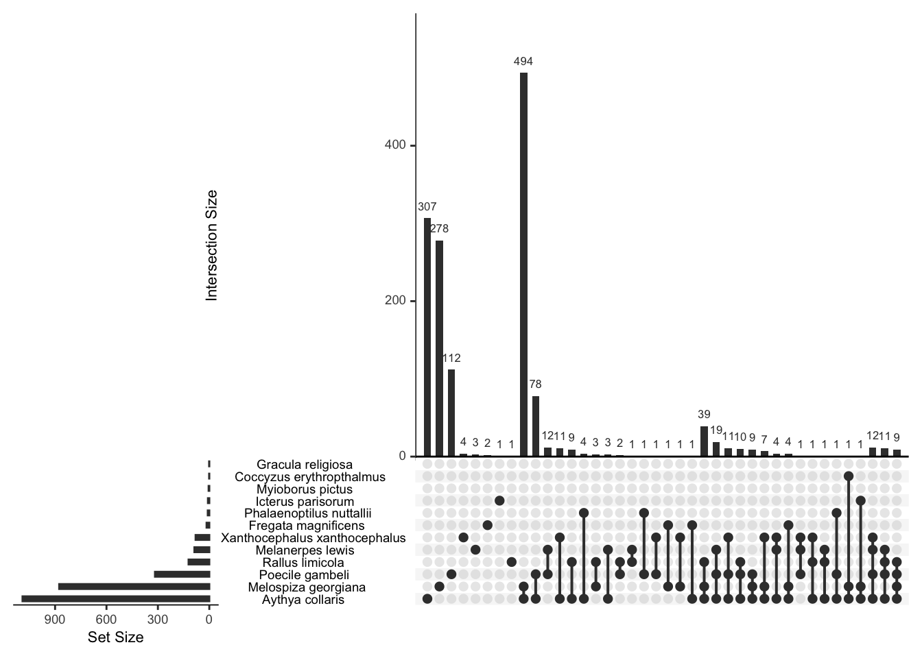
That’s all a bit clumsy because of the long names,but you can see, for example, that the swamp sparrow and ring-necked duck tend to co-occur. Let’s recode to shorter names.
bird_presence<-mr_recode(bird_presence,
  poorwill="Phalaenoptilus nuttallii",
  frigatebird="Fregata magnificens",
  woodpecker ="Melanerpes lewis",
  sparrow="Melospiza georgiana",
  rail="Rallus limicola",
  redstart="Myioborus pictus",
  chickadee="Poecile gambeli",
  duck="Aythya collaris",
  yellowhead="Xanthocephalus xanthocephalus",
  myna="Dracula religiosa",
  oriole="Icterus parisorum",
  cuckoo="Coccyzus erythropthalmus")
## Error in mr_recode(bird_presence, poorwill = "Phalaenoptilus nuttallii", : non-existent levels Dracula religiosaOops.
bird_presence<-mr_recode(bird_presence,
  poorwill="Phalaenoptilus nuttallii",
  frigatebird="Fregata magnificens",
  woodpecker ="Melanerpes lewis",
  sparrow="Melospiza georgiana",
  rail="Rallus limicola",
  redstart="Myioborus pictus",
  chickadee="Poecile gambeli",
  duck="Aythya collaris",
  yellowhead="Xanthocephalus xanthocephalus",
  myna="Gracula religiosa",
  oriole="Icterus parisorum",
  cuckoo="Coccyzus erythropthalmus")
Now try again:
mtable(bird_presence)## poorwill frigatebird woodpecker sparrow rail redstart chickadee duck
## 9 16 87 876 121 4 317 1090
## yellowhead myna oriole cuckoo
## 80 1 8 1mtable(bird_presence,bird_presence)## poorwill frigatebird woodpecker sparrow rail redstart
## poorwill 9 0 2 0 3 0
## frigatebird 0 16 0 12 8 0
## woodpecker 2 0 87 13 29 3
## sparrow 0 12 13 876 72 4
## rail 3 8 29 72 121 4
## redstart 0 0 3 4 4 4
## chickadee 5 0 72 34 52 3
## duck 8 13 70 593 114 4
## yellowhead 2 3 27 22 22 3
## myna 0 1 0 1 1 0
## oriole 0 0 4 5 4 3
## cuckoo 0 0 0 1 0 0
## chickadee duck yellowhead myna oriole cuckoo
## poorwill 5 8 2 0 0 0
## frigatebird 0 13 3 1 0 0
## woodpecker 72 70 27 0 4 0
## sparrow 34 593 22 1 5 1
## rail 52 114 22 1 4 0
## redstart 3 4 3 0 3 0
## chickadee 317 188 43 0 4 0
## duck 188 1090 73 1 7 1
## yellowhead 43 73 80 0 5 0
## myna 0 1 0 1 0 0
## oriole 4 7 5 0 8 0
## cuckoo 0 1 0 0 0 1plot(bird_presence, nsets=12,nint=30)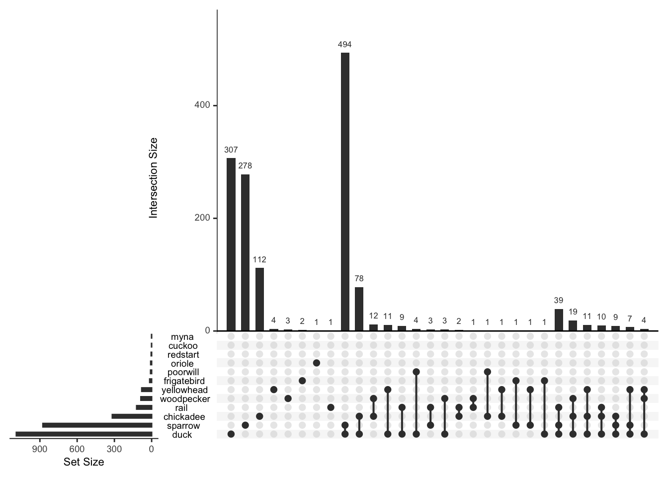
The default image plot is of the table of the variable by itself and shows the number of co-occurences. With type="conditional", the plot shows the proportion of each bird (on the y-axis) given that a particular bird (on the x-axis) is present.
image(bird_presence)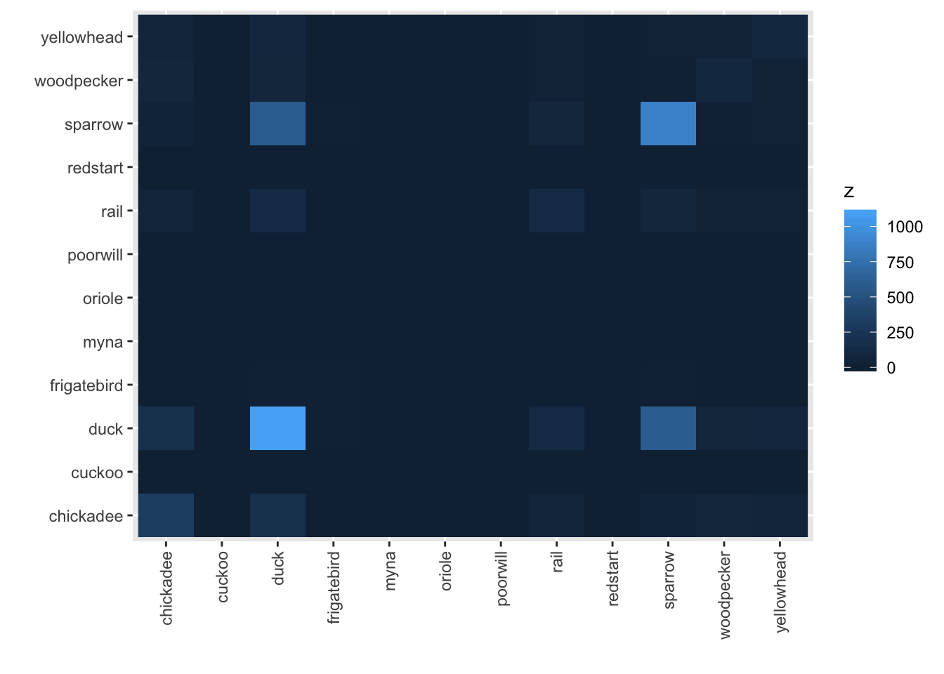
image(bird_presence, type="conditional")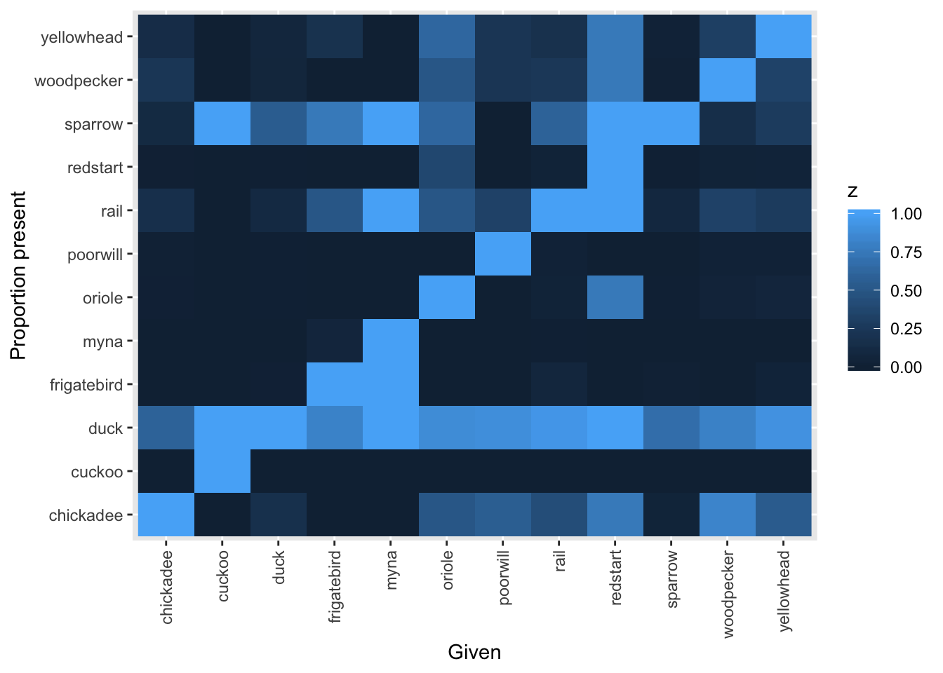
We might want to focus on just the more commonly observed birds
common_birds<-mr_lump(bird_presence,n=4)
mtable(common_birds)
## sparrow rail chickadee duck Other
## 876 121 317 1090 163mtable(common_birds,common_birds)## sparrow rail chickadee duck Other
## sparrow 876 72 34 593 44
## rail 72 121 52 114 48
## chickadee 34 52 317 188 97
## duck 593 114 188 1090 135
## Other 44 48 97 135 163plot(common_birds)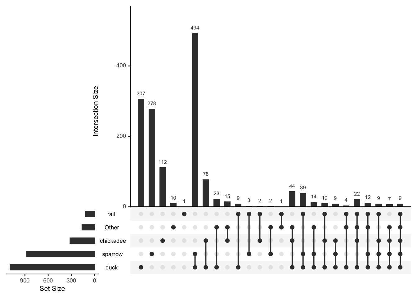
Or consider just the rare and interesting ones
rare_birds<-mr_lump(bird_presence,n=-5,other_level="Common")
mtable(rare_birds)
## poorwill redstart myna oriole cuckoo Common
## 9 4 1 8 1 1513mtable(rare_birds,rare_birds)## poorwill redstart myna oriole cuckoo Common
## poorwill 9 0 0 0 0 9
## redstart 0 4 0 3 0 4
## myna 0 0 1 0 0 1
## oriole 0 3 0 8 0 7
## cuckoo 0 0 0 0 1 1
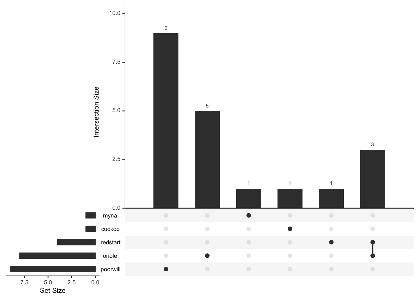
## Common 9 4 1 7 1 1513plot(rare_birds,nsets=6)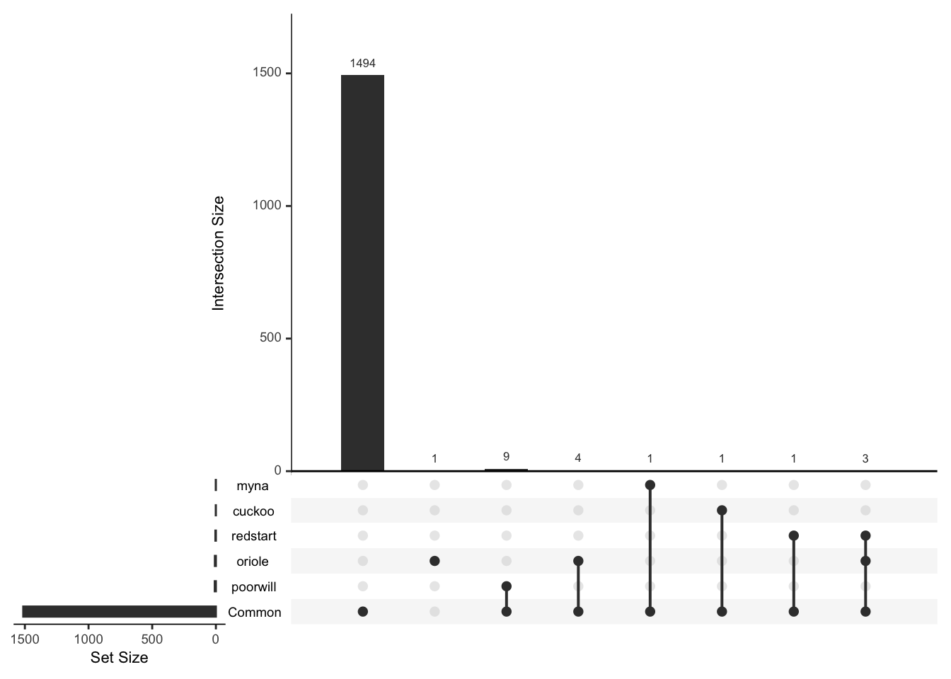
plot(mr_drop(rare_birds,"Common"),nsets=5)