One issue in teaching generalised linear models (or likelihood theory) is the relationship between the Wald, score, and likelihood ratio tests. I have a picture.
Let’s make up a score function \(U(\theta)\), in this case for a trivial binomial model, and draw it.
logit <-function(p) log(p/(1-p))
expit <-function(x) exp(x)/(1+exp(x))
U<-function(theta) 11/12-expit(theta)
thetahat<-logit(11/12)

curve( U(x),from=0, to =3, xlab=expression(theta),ylab=expression(U(theta)))
abline(h=0,lty=2)
abline(v=0,lty=2)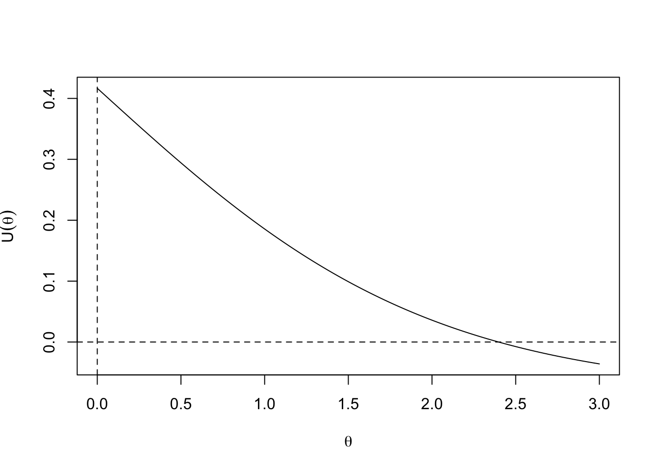
The likelihood ratio statistic is twice the area under the curve \[-2(\ell(\hat\theta)-\ell(0))= 2 \int_0^{\hat\theta}U(\theta)\,d\theta\]
curve( U(x),from=0, to =3, xlab=expression(theta),ylab=expression(U(theta)))
abline(h=0,lty=2)
abline(v=0,lty=2)
polygon(c(seq(0, thetahat,length=51),0), c(U(seq(0, thetahat,length=51)),0),col="#00000040")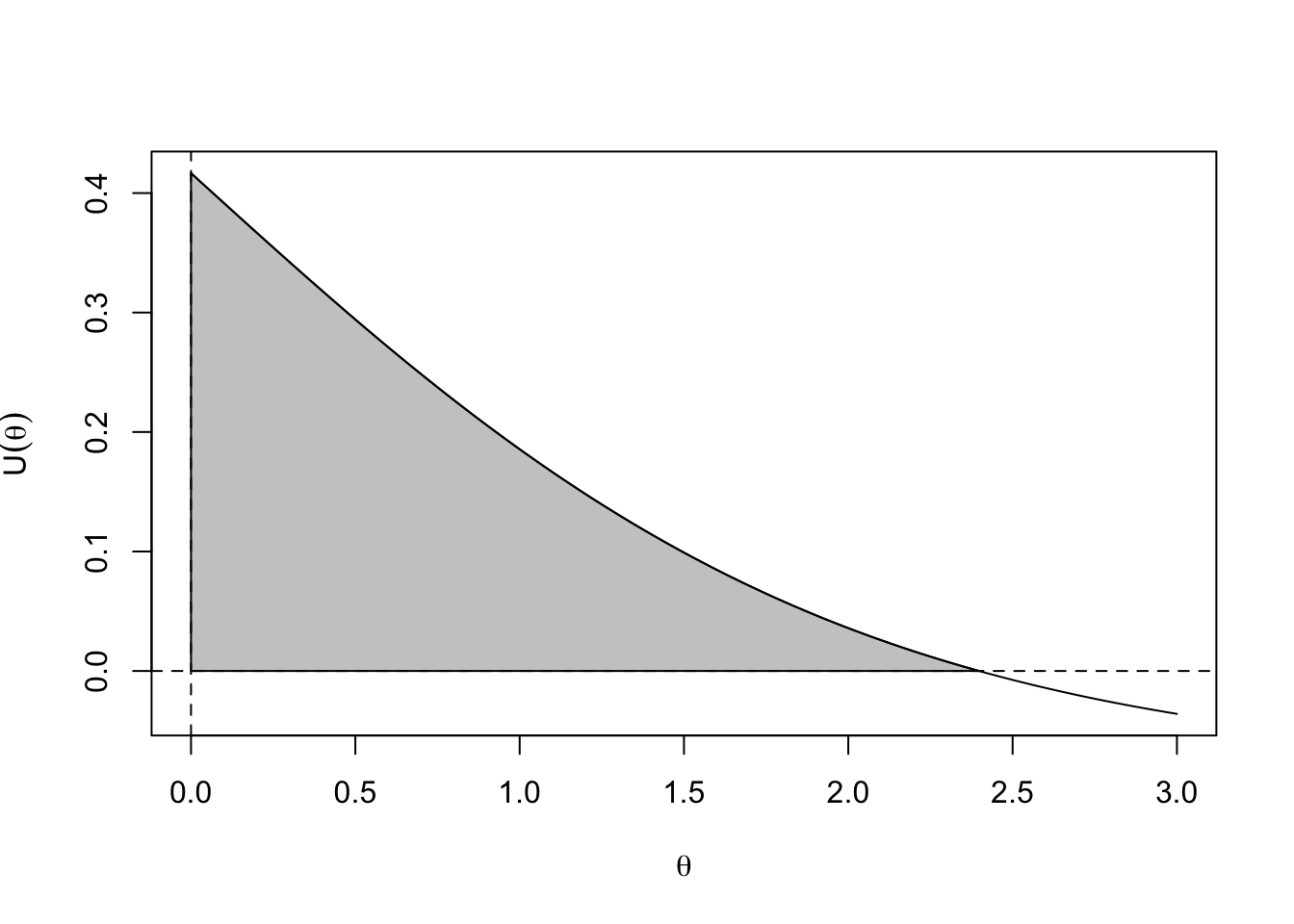
We can approximate this area by either of two triangles. One approximating triangle is tangent to the curve at \(\theta=0\)
Udot<-function(theta,d=0.001) (U(theta+d)-U(theta))/d

curve( U(x),from=0, to =3, xlab=expression(theta),ylab=expression(U(theta)))
abline(h=0,lty=2)
abline(v=0,lty=1,col="red")
abline(U(0),Udot(0),col="red")
polygon(x=c(0,0,-U(0)/Udot(0)),y=c(0,U(0),0), border=NA, col="#FF000060")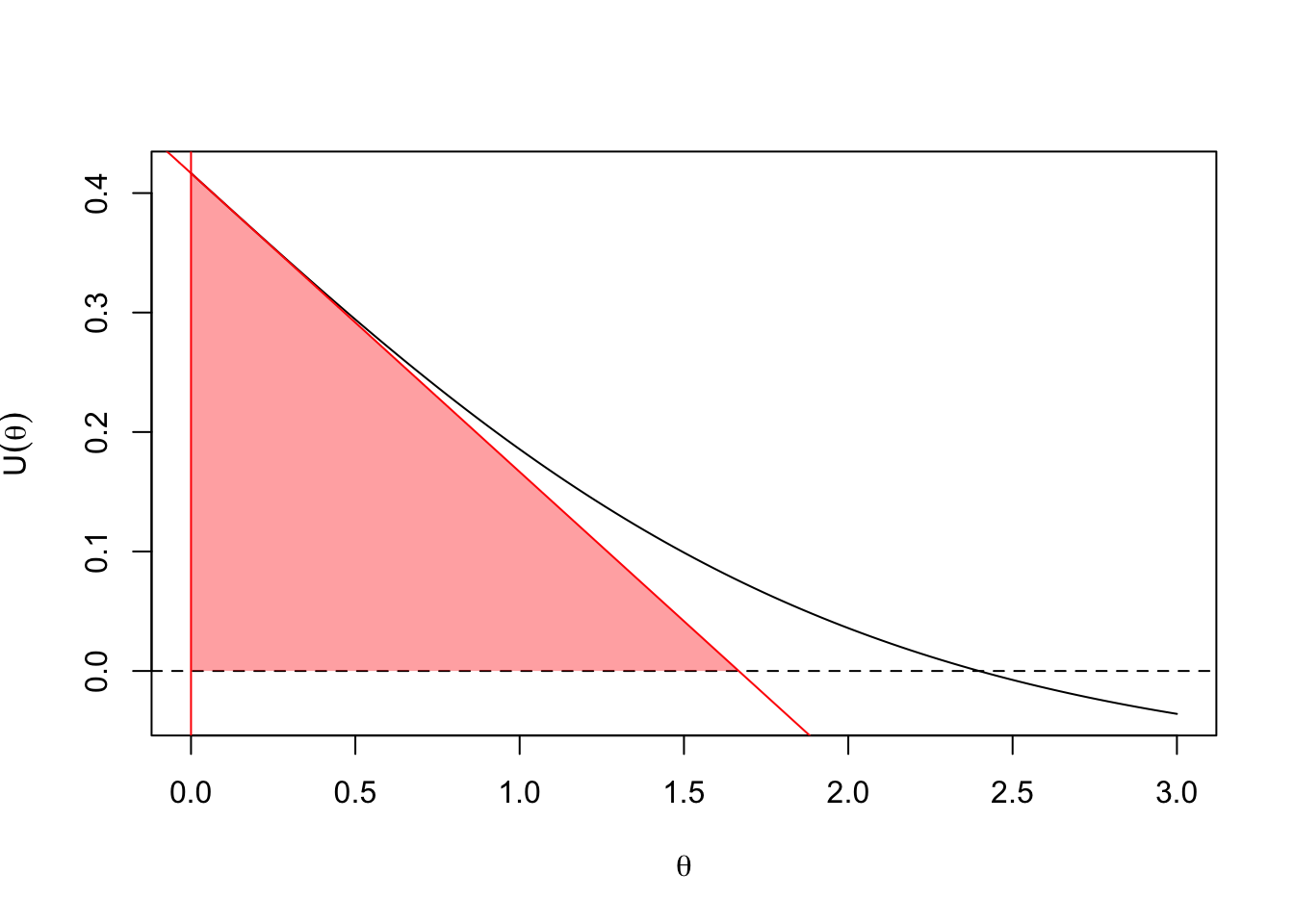
The red area is half the score test statistic: half of \(U(0)\times (U(0)/U'(0))\)
The other approximating triangle is tangent to the curve at \(\hat\theta\)
curve( U(x),from=0, to =3, xlab=expression(theta),ylab=expression(U(theta)))
abline(h=0,lty=1,col="royalblue")
abline(v=0,lty=2)
abline(-Udot(thetahat)*thetahat,Udot(thetahat),col="royalblue")
polygon(x=c(0,0,thetahat),y=c(0,-Udot(thetahat)*thetahat,0), border=NA, col="#0000FF60")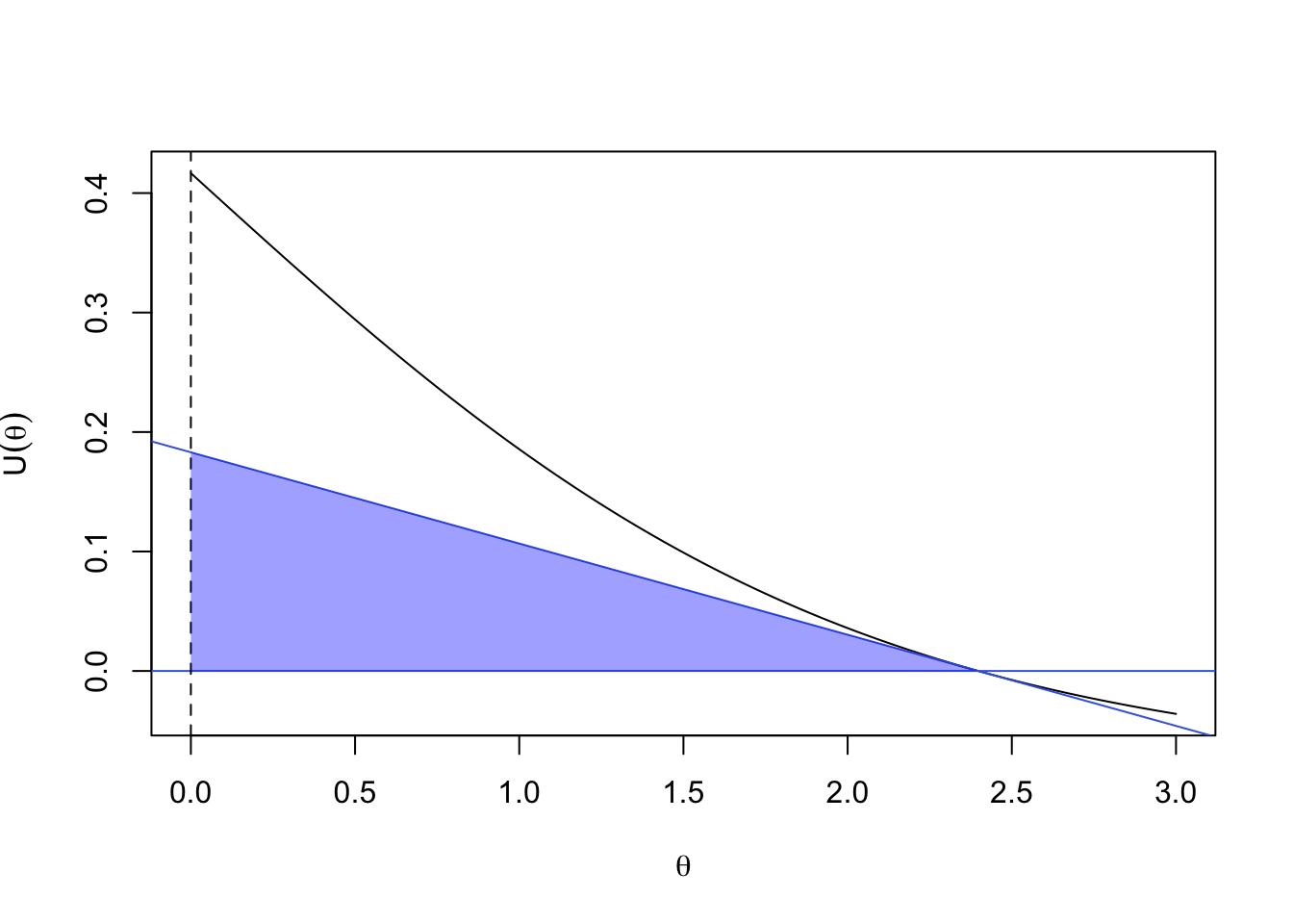
The blue area is half the Wald test statistic: half of \((\hat\theta U'(\hat\theta))\times \hat\theta\)
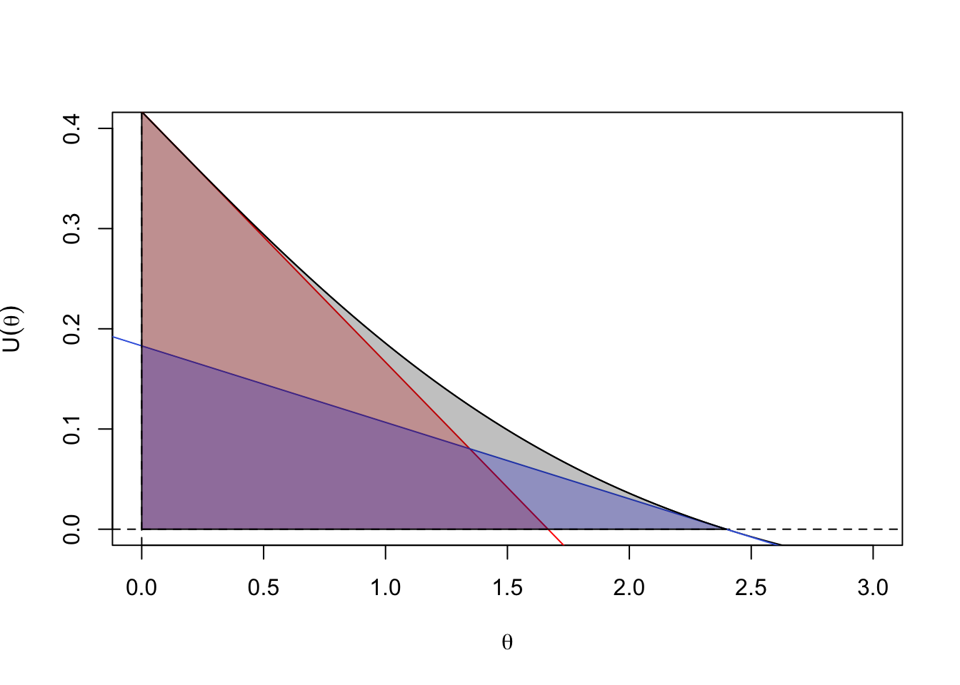
Here are all three of them together
curve( U(x),from=0, to =3, xlab=expression(theta),ylab=expression(U(theta)))
abline(h=0,lty=2)
abline(v=0,lty=2)
abline(U(0),Udot(0),col="red")
abline(-Udot(thetahat)*thetahat,Udot(thetahat),col="royalblue")
polygon(x=c(0,0,-U(0)/Udot(0)),y=c(0,U(0),0), border=NA, col="#FF000040")
polygon(x=c(0,0,thetahat),y=c(0,-Udot(thetahat)*thetahat,0), border=NA, col="#0000FF40")
polygon(c(seq(0, thetahat,length=51),0), c(U(seq(0, thetahat,length=51)),0),col="#00000040")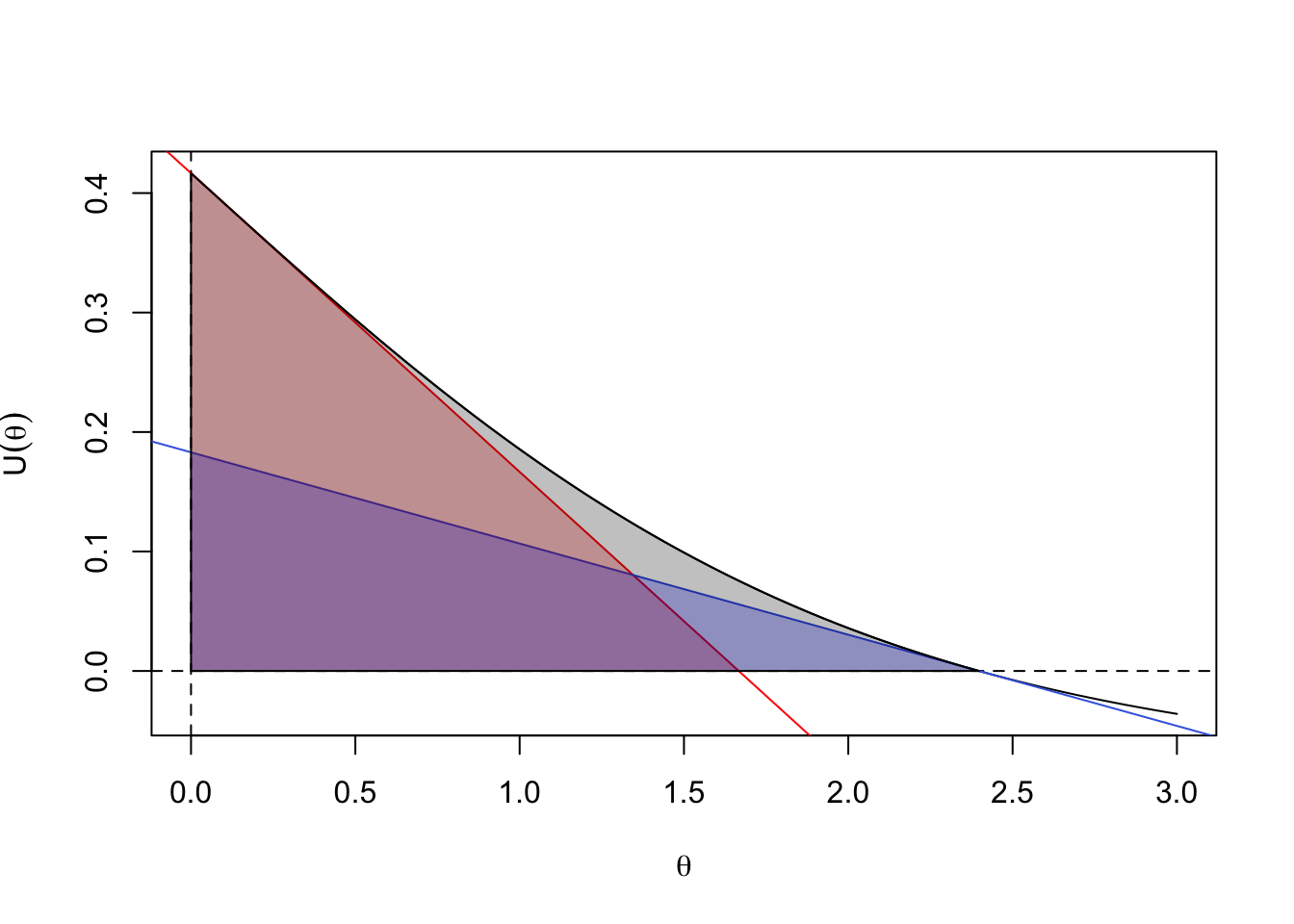
Under local alternatives, when \(\hat\theta\) approaches \(\theta_0\) the curve \(U(\theta)\) will straighten out (by Taylor’s Theorem) and the three areas will be closer together
U<-function(theta) 8/14-expit(theta)
thetahat<-logit(8/14)
curve( U(x),from=0, to =0.3, xlab=expression(theta),ylab=expression(U(theta)))
abline(h=0,lty=2)
abline(v=0,lty=2)
abline(U(0),Udot(0),col="red")
abline(-Udot(thetahat)*thetahat,Udot(thetahat),col="royalblue")
polygon(x=c(0,0,-U(0)/Udot(0)),y=c(0,U(0),0), border=NA, col="#FF000040")
polygon(x=c(0,0,thetahat),y=c(0,-Udot(thetahat)*thetahat,0), border=NA, col="#0000FF40")
polygon(c(seq(0, thetahat,length=51),0), c(U(seq(0, thetahat,length=51)),0),col="#00000040")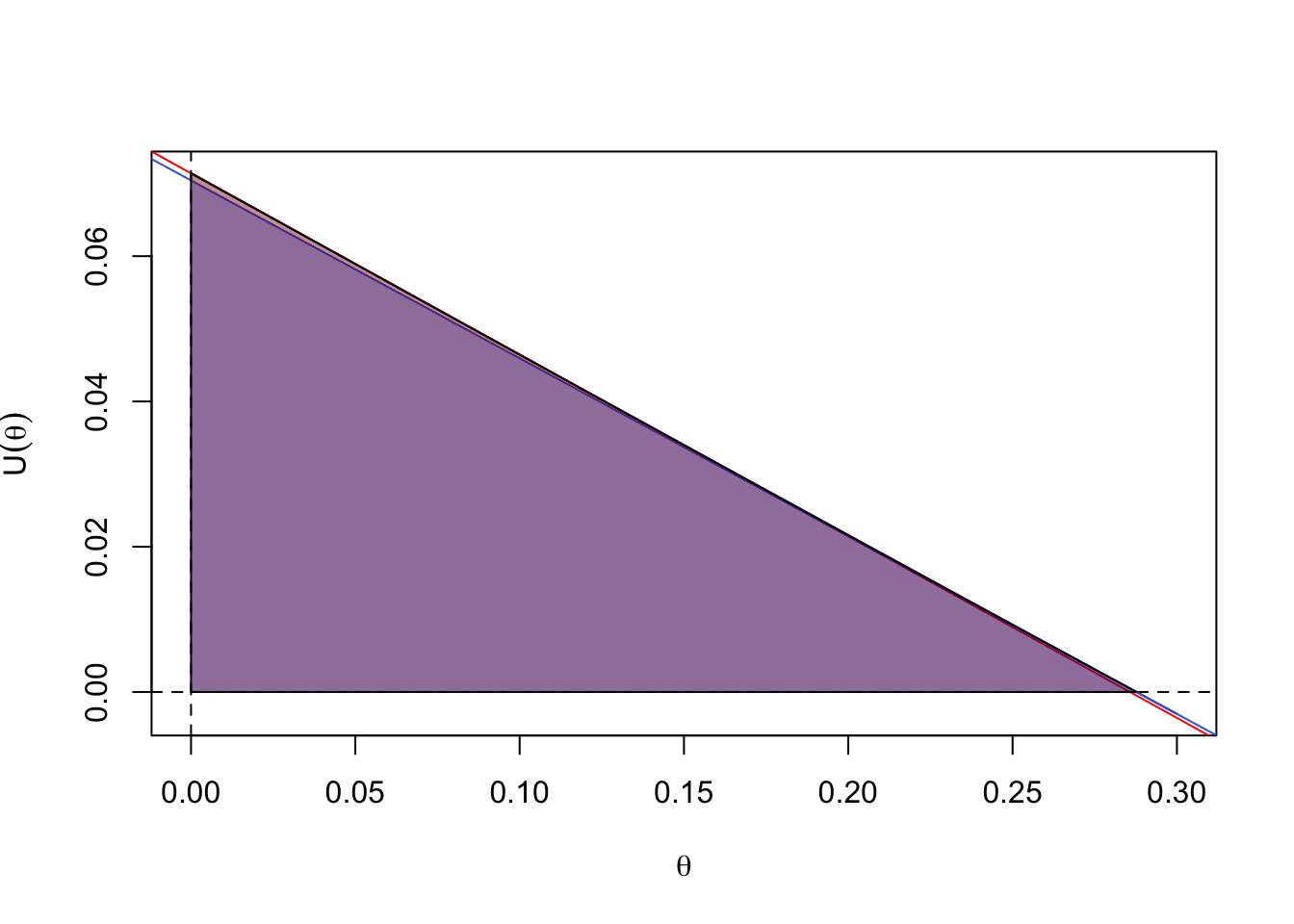
But under fixed alternatives this isn’t guaranteed even at large sample size:
U<-function(theta) 110/120-expit(theta)
thetahat<-logit(110/120)
curve( U(x),from=0, to =3, xlab=expression(theta),ylab=expression(U(theta)),ylim=c(0,.4))
abline(h=0,lty=2)
abline(v=0,lty=2)
abline(U(0),Udot(0),col="red")
abline(-Udot(thetahat)*thetahat,Udot(thetahat),col="royalblue")
polygon(x=c(0,0,-U(0)/Udot(0)),y=c(0,U(0),0), border=NA, col="#FF000040")
polygon(x=c(0,0,thetahat),y=c(0,-Udot(thetahat)*thetahat,0), border=NA, col="#0000FF40")
polygon(c(seq(0, thetahat,length=51),0), c(U(seq(0, thetahat,length=51)),0),col="#00000040")