The issue
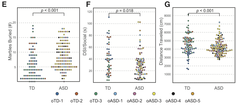
A paper reporting the induction of autism-type behaviour in mice by fecal microbiome transplants from humans was recently published in Cell. Some people on Twitter were discussing subplots E, F, and G of Figure 1, which report behavioral comparisons of the mice between fecal donors with and without ASD.

The expressed view on Twitter was the the plots weren’t consistent with the \(p\)-values given. They didn’t entirely need to be, since the \(p\)-values weren’t from a simple two-group comparison, but even taking that into account I was surprised. I thought it was worth doing the actual comparison the researchers reported before going all ‘someone is wrong on the internet’ about it. That turned out to be relatively tricky.
The data
The data are available from https://doi.org/10.17632/ngzmj4zkms. I downloaded the data for Figure 1, parts E–H.
cell<-read.csv("https://data.mendeley.com/datasets/ngzmj4zkms/1/files/fb7927df-a1ea-4257-bf2f-33fecc4090e9/Fig1EFGH_subset8.csv?dl=1")First, check the plots to make sure the data look right
library(beeswarm)
cell$ASD_diagnosis<-relevel(cell$ASD_diagnosis, ref="NT")
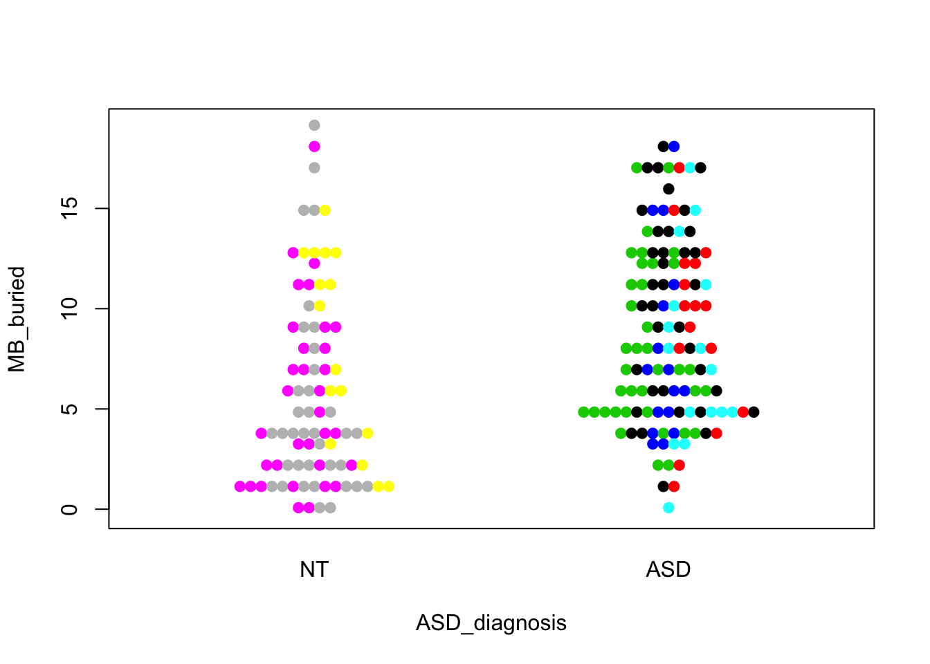
beeswarm(MB_buried~ASD_diagnosis,data=cell,method="center",pch=19,pwcol=Donor)
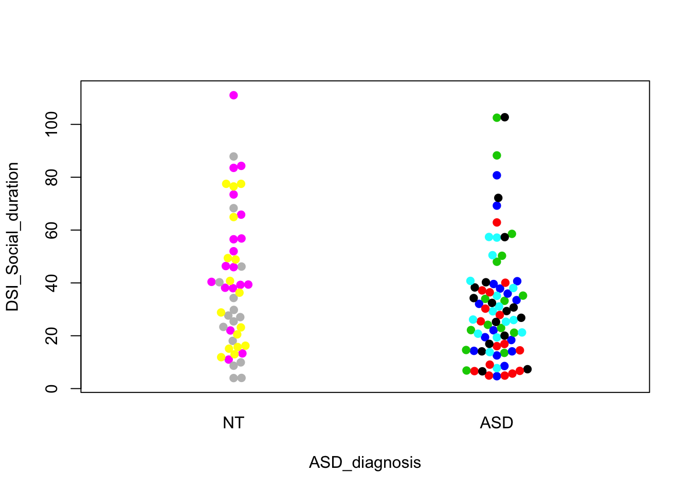
beeswarm(DSI_Social_duration~ASD_diagnosis,data=cell,pch=19,pwcol=Donor)
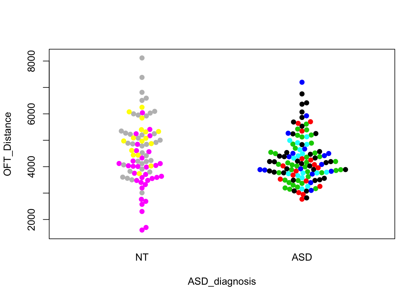
beeswarm(OFT_Distance~ASD_diagnosis,data=cell,pch=19,pwcol=Donor)
These look like the ones in the paper. The first one shows a visually convincing difference; the other two do not. We can easily do formal tests that correspond to these visual comparisons
t.test(MB_buried~ASD_diagnosis,data=cell)##
## Welch Two Sample t-test
##
## data: MB_buried by ASD_diagnosis
## t = -4.5452, df = 172.79, p-value = 1.028e-05
## alternative hypothesis: true difference in means is not equal to 0
## 95 percent confidence interval:
## -4.279629 -1.688091
## sample estimates:
## mean in group NT mean in group ASD
## 5.776471 8.760331t.test(DSI_Social_duration~ASD_diagnosis,data=cell)##
## Welch Two Sample t-test
##
## data: DSI_Social_duration by ASD_diagnosis
## t = 2.1568, df = 88.93, p-value = 0.03372
## alternative hypothesis: true difference in means is not equal to 0
## 95 percent confidence interval:
## 0.7446561 18.1694410
## sample estimates:
## mean in group NT mean in group ASD
## 40.57806 31.12101t.test(OFT_Distance~ASD_diagnosis,data=cell)##
## Welch Two Sample t-test
##
## data: OFT_Distance by ASD_diagnosis
## t = 1.9731, df = 144.85, p-value = 0.05039
## alternative hypothesis: true difference in means is not equal to 0
## 95 percent confidence interval:
## -0.5077242 592.3180052
## sample estimates:
## mean in group NT mean in group ASD
## 4548.462 4252.557However, the aggregate comparison is wrong. The researchers say in the panel caption that “Hypothesis testing for differences of the means were done by a mixed effects analysis using donor diagnosis and mouse sex as fixed effects and donor ID as a random effect.”
That’s a plausible analysis. So let’s do it. I’ll use lmer, with the lmerTest package to get small-sample approximations.
library(lmerTest)## Loading required package: lme4## Loading required package: Matrix## Registered S3 methods overwritten by 'ggplot2':
## method from
## [.quosures rlang
## c.quosures rlang
## print.quosures rlang##
## Attaching package: 'lmerTest'## The following object is masked from 'package:lme4':
##
## lmer## The following object is masked from 'package:stats':
##
## stepmarbles<-lmer(MB_buried~ASD_diagnosis+Gender+(1|Donor),data=cell)
dsi<-lmer(DSI_Social_duration~ASD_diagnosis+Gender+(1|Donor),data=cell)
oft<-lmer(OFT_Distance~ASD_diagnosis+Gender+(1|Donor),data=cell)
summary(marbles)## Linear mixed model fit by REML. t-tests use Satterthwaite's method [
## lmerModLmerTest]
## Formula: MB_buried ~ ASD_diagnosis + Gender + (1 | Donor)
## Data: cell
##
## REML criterion at convergence: 1203.4
##
## Scaled residuals:
## Min 1Q Median 3Q Max
## -1.8852 -0.8420 -0.1855 0.7049 2.8853
##
## Random effects:
## Groups Name Variance Std.Dev.
## Donor (Intercept) 0.8052 0.8973
## Residual 20.1949 4.4939
## Number of obs: 206, groups: Donor, 8
##
## Fixed effects:
## Estimate Std. Error df t value Pr(>|t|)
## (Intercept) 6.5928 0.7950 7.7089 8.293 4.18e-05 ***
## ASD_diagnosisASD 2.6777 0.9292 5.5842 2.882 0.0304 *
## GenderMale -1.2002 0.6315 201.1337 -1.901 0.0588 .
## ---
## Signif. codes: 0 '***' 0.001 '**' 0.01 '*' 0.05 '.' 0.1 ' ' 1
##
## Correlation of Fixed Effects:
## (Intr) ASD_AS
## ASD_dgnsASD -0.718
## GenderMale -0.420 0.031summary(dsi)## Linear mixed model fit by REML. t-tests use Satterthwaite's method [
## lmerModLmerTest]
## Formula: DSI_Social_duration ~ ASD_diagnosis + Gender + (1 | Donor)
## Data: cell
##
## REML criterion at convergence: 1109.7
##
## Scaled residuals:
## Min 1Q Median 3Q Max
## -1.8408 -0.7024 -0.1325 0.6461 3.0087
##
## Random effects:
## Groups Name Variance Std.Dev.
## Donor (Intercept) 22.32 4.724
## Residual 369.96 19.234
## Number of obs: 128, groups: Donor, 8
##
## Fixed effects:
## Estimate Std. Error df t value Pr(>|t|)
## (Intercept) 27.064 4.303 8.919 6.290 0.000148 ***
## ASD_diagnosisASD -8.097 4.917 5.948 -1.647 0.151138
## GenderMale 24.082 3.418 120.475 7.045 1.24e-10 ***
## ---
## Signif. codes: 0 '***' 0.001 '**' 0.01 '*' 0.05 '.' 0.1 ' ' 1
##
## Correlation of Fixed Effects:
## (Intr) ASD_AS
## ASD_dgnsASD -0.722
## GenderMale -0.435 0.029summary(oft)## Linear mixed model fit by REML. t-tests use Satterthwaite's method [
## lmerModLmerTest]
## Formula: OFT_Distance ~ ASD_diagnosis + Gender + (1 | Donor)
## Data: cell
##
## REML criterion at convergence: 3375.2
##
## Scaled residuals:
## Min 1Q Median 3Q Max
## -2.5439 -0.6125 -0.1220 0.4504 3.3174
##
## Random effects:
## Groups Name Variance Std.Dev.
## Donor (Intercept) 166783 408.4
## Residual 867930 931.6
## Number of obs: 206, groups: Donor, 8
##
## Fixed effects:
## Estimate Std. Error df t value Pr(>|t|)
## (Intercept) 4658.881 267.832 7.003 17.395 5.08e-07 ***
## ASD_diagnosisASD -369.892 329.402 6.256 -1.123 0.303
## GenderMale -111.803 131.383 198.647 -0.851 0.396
## ---
## Signif. codes: 0 '***' 0.001 '**' 0.01 '*' 0.05 '.' 0.1 ' ' 1
##
## Correlation of Fixed Effects:
## (Intr) ASD_AS
## ASD_dgnsASD -0.763
## GenderMale -0.259 0.017anova(marbles)## Type III Analysis of Variance Table with Satterthwaite's method
## Sum Sq Mean Sq NumDF DenDF F value Pr(>F)
## ASD_diagnosis 167.713 167.713 1 5.584 8.3047 0.03037 *
## Gender 72.953 72.953 1 201.134 3.6124 0.05878 .
## ---
## Signif. codes: 0 '***' 0.001 '**' 0.01 '*' 0.05 '.' 0.1 ' ' 1anova(dsi)## Type III Analysis of Variance Table with Satterthwaite's method
## Sum Sq Mean Sq NumDF DenDF F value Pr(>F)
## ASD_diagnosis 1003.3 1003.3 1 5.948 2.7119 0.1511
## Gender 18364.3 18364.3 1 120.475 49.6382 1.241e-10 ***
## ---
## Signif. codes: 0 '***' 0.001 '**' 0.01 '*' 0.05 '.' 0.1 ' ' 1anova(oft)## Type III Analysis of Variance Table with Satterthwaite's method
## Sum Sq Mean Sq NumDF DenDF F value Pr(>F)
## ASD_diagnosis 1094412 1094412 1 6.256 1.2609 0.3027
## Gender 628519 628519 1 198.647 0.7242 0.3958Taking account of within-donor correlation reduces the effective sample size and the standard errors get much bigger. There’s modest evidence for the marbles, but basically none for the other outcomes. We could redo with the (slightly improved) Kenward-Roger version of the anova tests.
anova(marbles, ddf="Kenward-Roger")## Type III Analysis of Variance Table with Kenward-Roger's method
## Sum Sq Mean Sq NumDF DenDF F value Pr(>F)
## ASD_diagnosis 163.812 163.812 1 5.331 8.1115 0.03339 *
## Gender 72.224 72.224 1 201.044 3.5764 0.06005 .
## ---
## Signif. codes: 0 '***' 0.001 '**' 0.01 '*' 0.05 '.' 0.1 ' ' 1anova(dsi, ddf="Kenward-Roger")## Type III Analysis of Variance Table with Kenward-Roger's method
## Sum Sq Mean Sq NumDF DenDF F value Pr(>F)
## ASD_diagnosis 1002.7 1002.7 1 5.932 2.7103 0.1514
## Gender 18279.3 18279.3 1 120.459 49.4084 1.349e-10 ***
## ---
## Signif. codes: 0 '***' 0.001 '**' 0.01 '*' 0.05 '.' 0.1 ' ' 1anova(oft, ddf="Kenward-Roger")## Type III Analysis of Variance Table with Kenward-Roger's method
## Sum Sq Mean Sq NumDF DenDF F value Pr(>F)
## ASD_diagnosis 1090931 1090931 1 5.829 1.2569 0.3063
## Gender 626912 626912 1 198.326 0.7223 0.3964Still unimpressive.
If we look at the statistical analysis section at the end of the paper it says “Comparison of behavioral outcomes between TD Controls and ASD donors were tested using longitudinal linear mixed effects analyses, with test cycles and donors treated as repeated factors. Analyses were performed in SPSS (v 24);a priori alpha = 0.05. All outcomes were tested for normality and trans-formed as required. Diagonal covariance matrices were used so that intra-cycle and intra-donor correlations were accounted for inthe modeling.”
I’m not sure quite what that means– mice don’t repeat over donors or cycles– but it would make sense to have a Cycle effect for the marbles and OFT analyses; the DSI was only done in one cycle, so there can’t be a “cycle effect”. The impact shouldn’t be huge, since cycle is roughly orthogonal to ASD. With only two cycles, I would have made it a fixed effect, but we can try either way.
library(lmerTest)
marbles<-lmer(MB_buried~ASD_diagnosis+Gender+(1|Cycle)+(1|Donor),data=cell)
## Warning in checkConv(attr(opt, "derivs"), opt$par, ctrl =
## control$checkConv, : Model failed to converge with max|grad| = 0.0219471
## (tol = 0.002, component 1)oft<-lmer(OFT_Distance~ASD_diagnosis+Gender+(1|Cycle)+(1|Donor),data=cell)
anova(marbles, ddf="Kenward-Roger")## Type III Analysis of Variance Table with Kenward-Roger's method
## Sum Sq Mean Sq NumDF DenDF F value Pr(>F)
## ASD_diagnosis 160.758 160.758 1 5.315 7.9603 0.03461 *
## Gender 70.849 70.849 1 201.039 3.5083 0.06252 .
## ---
## Signif. codes: 0 '***' 0.001 '**' 0.01 '*' 0.05 '.' 0.1 ' ' 1anova(oft, ddf="Kenward-Roger")## Type III Analysis of Variance Table with Kenward-Roger's method
## Sum Sq Mean Sq NumDF DenDF F value Pr(>F)
## ASD_diagnosis 1054021 1054021 1 5.808 1.2162 0.3137
## Gender 593327 593327 1 198.253 0.6846 0.4090marbles2<-lmer(MB_buried~ASD_diagnosis+Gender+Cycle+(1|Donor),data=cell)
oft2<-lmer(OFT_Distance~ASD_diagnosis+Gender+Cycle+(1|Donor),data=cell)
anova(marbles2, ddf="Kenward-Roger")## Type III Analysis of Variance Table with Kenward-Roger's method
## Sum Sq Mean Sq NumDF DenDF F value Pr(>F)
## ASD_diagnosis 156.791 156.791 1 5.138 7.7419 0.03766 *
## Gender 70.145 70.145 1 199.850 3.4636 0.06420 .
## Cycle 2.978 2.978 1 127.464 0.1471 0.70199
## ---
## Signif. codes: 0 '***' 0.001 '**' 0.01 '*' 0.05 '.' 0.1 ' ' 1anova(oft2, ddf="Kenward-Roger")## Type III Analysis of Variance Table with Kenward-Roger's method
## Sum Sq Mean Sq NumDF DenDF F value Pr(>F)
## ASD_diagnosis 949822 949822 1 5.741 1.0971 0.3370
## Gender 511565 511565 1 197.269 0.5909 0.4430
## Cycle 1054078 1054078 1 194.334 1.2175 0.2712And it doesn’t matter much.
The Statistical analysis section also says “Additional statistical analysis was done using R (3.4.1) or Python (3.6.4), using various packages to test mixed effects testing diagnosis (TD or ASD) as a fixed effect and donor and testing round as random effects.”. I think ‘various packages’ is a bit unspecific, but let’s try Round as a random effect.
library(lmerTest)
marbles<-lmer(MB_buried~ASD_diagnosis+Gender+(1|Round)+(1|Donor),data=cell)
## boundary (singular) fit: see ?isSingulardsi<-lmer(DSI_Social_duration~ASD_diagnosis+Gender+(1|Round)+(1|Donor),data=cell)## boundary (singular) fit: see ?isSingularoft<-lmer(OFT_Distance~ASD_diagnosis+Gender+(1|Round)+(1|Donor),data=cell)
anova(marbles, ddf="Kenward-Roger")## Type III Analysis of Variance Table with Kenward-Roger's method
## Sum Sq Mean Sq NumDF DenDF F value Pr(>F)
## ASD_diagnosis 156.844 156.844 1 5.189 7.7666 0.03705 *
## Gender 70.447 70.447 1 200.926 3.4884 0.06326 .
## ---
## Signif. codes: 0 '***' 0.001 '**' 0.01 '*' 0.05 '.' 0.1 ' ' 1anova(dsi, ddf="Kenward-Roger")## Type III Analysis of Variance Table with Kenward-Roger's method
## Sum Sq Mean Sq NumDF DenDF F value Pr(>F)
## ASD_diagnosis 738.4 738.4 1 5.597 1.9957 0.2109
## Gender 18228.0 18228.0 1 120.455 49.2689 1.419e-10 ***
## ---
## Signif. codes: 0 '***' 0.001 '**' 0.01 '*' 0.05 '.' 0.1 ' ' 1anova(oft, ddf="Kenward-Roger")## Type III Analysis of Variance Table with Kenward-Roger's method
## Sum Sq Mean Sq NumDF DenDF F value Pr(>F)
## ASD_diagnosis 853223 853223 1 4.847 1.0655 0.3507
## Gender 901440 901440 1 196.177 1.1257 0.2900Again, not much change. (The warning message is harmless: it jut means that that Round random effect is estimated to have zero variance.)
There’s an Excel spreadsheet with test statistics and p-values as table S4. It doesn’t say exactly what the tests were, and I don’t have access to SPSS on a holiday long weekend, but there are two notable things about it. First, it has interaction p-values for Diagnosis by Gender. Second, the F statistics for Diagnosis have 169, 79, and 95 denominator degrees of freedom for the marbles, DSI, and OFT outcomes respectively.
Information for the Diagnosis contrast only comes from comparisons between the 5 donor humans with ASD and the 3 donor controls, so the degrees of freedom should be no more than 7, and probably less.
Let’s try one more time, though, with a sex by diagnosis interaction:
library(lmerTest)
marbles<-lmer(MB_buried~ASD_diagnosis*Gender+(1|Round)+(1|Donor),data=cell)
## boundary (singular) fit: see ?isSingulardsi<-lmer(DSI_Social_duration~ASD_diagnosis*Gender+(1|Round)+(1|Donor),data=cell)## boundary (singular) fit: see ?isSingularoft<-lmer(OFT_Distance~ASD_diagnosis*Gender+(1|Round)+(1|Donor),data=cell)
anova(marbles, ddf="Kenward-Roger")## Type III Analysis of Variance Table with Kenward-Roger's method
## Sum Sq Mean Sq NumDF DenDF F value Pr(>F)
## ASD_diagnosis 159.509 159.509 1 5.135 7.9685 0.03590 *
## Gender 92.203 92.203 1 200.360 4.6061 0.03306 *
## ASD_diagnosis:Gender 58.626 58.626 1 200.073 2.9287 0.08857 .
## ---
## Signif. codes: 0 '***' 0.001 '**' 0.01 '*' 0.05 '.' 0.1 ' ' 1anova(dsi, ddf="Kenward-Roger")## Type III Analysis of Variance Table with Kenward-Roger's method
## Sum Sq Mean Sq NumDF DenDF F value Pr(>F)
## ASD_diagnosis 736.2 736.2 1 5.595 1.9838 0.2121
## Gender 18289.0 18289.0 1 120.347 49.2836 1.416e-10 ***
## ASD_diagnosis:Gender 338.6 338.6 1 120.323 0.9126 0.3414
## ---
## Signif. codes: 0 '***' 0.001 '**' 0.01 '*' 0.05 '.' 0.1 ' ' 1anova(oft, ddf="Kenward-Roger")## Type III Analysis of Variance Table with Kenward-Roger's method
## Sum Sq Mean Sq NumDF DenDF F value Pr(>F)
## ASD_diagnosis 850027 850027 1 4.844 1.0565 0.3526
## Gender 823622 823622 1 195.277 1.0237 0.3129
## ASD_diagnosis:Gender 23723 23723 1 194.337 0.0295 0.8638and, finally, using sum-to-zero contrasts instead of treatment contrasts
library(lmerTest)
cell$ASD_sum<-C(cell$ASD_diagnosis,"contr.sum")
cell$Gender_sum<-C(cell$Gender,"contr.sum")
marbles<-lmer(MB_buried~ASD_sum*Gender_sum+(1|Round)+(1|Donor),data=cell)
## boundary (singular) fit: see ?isSingulardsi<-lmer(DSI_Social_duration~ASD_sum*Gender_sum+(1|Round)+(1|Donor),data=cell)## boundary (singular) fit: see ?isSingularoft<-lmer(OFT_Distance~ASD_sum*Gender_sum+(1|Round)+(1|Donor),data=cell)
anova(marbles, ddf="Kenward-Roger")## Type III Analysis of Variance Table with Kenward-Roger's method
## Sum Sq Mean Sq NumDF DenDF F value Pr(>F)
## ASD_sum 159.509 159.509 1 5.135 7.9685 0.03590 *
## Gender_sum 92.203 92.203 1 200.360 4.6061 0.03306 *
## ASD_sum:Gender_sum 58.626 58.626 1 200.073 2.9287 0.08857 .
## ---
## Signif. codes: 0 '***' 0.001 '**' 0.01 '*' 0.05 '.' 0.1 ' ' 1anova(dsi, ddf="Kenward-Roger")## Type III Analysis of Variance Table with Kenward-Roger's method
## Sum Sq Mean Sq NumDF DenDF F value Pr(>F)
## ASD_sum 736.2 736.2 1 5.595 1.9838 0.2121
## Gender_sum 18289.0 18289.0 1 120.347 49.2836 1.416e-10 ***
## ASD_sum:Gender_sum 338.6 338.6 1 120.323 0.9126 0.3414
## ---
## Signif. codes: 0 '***' 0.001 '**' 0.01 '*' 0.05 '.' 0.1 ' ' 1anova(oft, ddf="Kenward-Roger")## Type III Analysis of Variance Table with Kenward-Roger's method
## Sum Sq Mean Sq NumDF DenDF F value Pr(>F)
## ASD_sum 850027 850027 1 4.844 1.0565 0.3526
## Gender_sum 823622 823622 1 195.277 1.0237 0.3129
## ASD_sum:Gender_sum 23723 23723 1 194.337 0.0295 0.8638So, in the end I can’t reproduce anything close to the \(p\)-values given in the paper. I suspect based on the analyses I’ve done and the degrees of freedom given in the paper that the \(p\)-values in the paper are wrong. However, since I can’t come close to reproducing them, I can’t be sure.
Given that the authors were clearly computationally literate and familiar with mixed model software in R, it’s a pity these analyses weren’t done in R (or Python or something) so that code could be distributed with the data.
A New Hope
I tried to work out what the SPSS commands reported in the paper might be doing, in particular the bit about “diagonal covariance matrices”. SPSS has an option for “Diagonal” in specifying within-subject covariance matrices, which models heteroscedasticity but not correlation. If you already had random effects in the model that would be what you wanted, but if you didn’t it would end up treating all the observations as independent.
It’s a new day, and I could try this with a copy of SPSS. Now I can duplicate the test statistics and p-values exactly with the following SPSS syntax (generated by the SPSS GUI)
MIXED OFT_Distance BY Gender ASD_diagnosis
  /CRITERIA=CIN(95) MXITER(100) MXSTEP(10) SCORING(1) SINGULAR(0.000000000001) HCONVERGE(0,
    ABSOLUTE) LCONVERGE(0, ABSOLUTE) PCONVERGE(0.000001, ABSOLUTE)
  /FIXED=Gender ASD_diagnosis Gender*ASD_diagnosis | SSTYPE(3)
  /METHOD=REML
  /REPEATED=Donor | SUBJECT(V1) COVTYPE(DIAG)
and then replacing OFT_Distance with MB_buried or DSI_Social_duration.
The output in SPSS is like this (only pretty)
    Type III Tests of Fixed Effects a
Source          Numerator df    Denominator df  F         Sig.
Intercept                 1           95.967      4336.047  .000
Gender                  1           95.967       2.378  .126
ASD_diagnosis             1         95.967      15.346  .000
Gender * ASD_diagnosis  1           95.967       1.871  .175
a Dependent Variable: OFT_Distance.
This, as far as I can tell from the documentation, is a regression model with all observations independent, but with the variance depending on Donor. Which is not an analysis I would consider to be appropriate. To get a random effect of donor in SPSS, you’d use a /RANDOM = Donor line.
I can at least approximately get this analysis in R using gls. There are a lot of details in how these models are fitted, and SPSS and R’s gls have differences. But the model it fits is the one I think SPSS is fitting and the results for the \(F\)-statistics are almost identical. The degrees of freedom are off, and therefore the p-values aren’t the same, because gls uses a much cruder df computation. However, the p-values are close because the analysis (incorrectly) specifies that there are lots and lots of denominator degrees of freedom: the difference between 95 and 202 doesn’t make much difference.
library(nlme)##
## Attaching package: 'nlme'## The following object is masked from 'package:lme4':
##
## lmListcell$ASD_sum<-C(cell$ASD_diagnosis,"contr.sum")
cell$Gender_sum<-C(cell$Gender,"contr.sum")
marbles_gls <- gls(MB_buried~ASD_sum*Gender_sum, weights=varIdent(form=~1|Donor),data=cell)
dsi_gls <- gls(DSI_Social_duration~ASD_sum*Gender_sum, weights=varIdent(form=~1|Donor),data=cell,na.action=na.omit)
oft_gls <- gls(OFT_Distance~ASD_sum*Gender_sum, weights=varIdent(form=~1|Donor),data=cell)
marbles_gls## Generalized least squares fit by REML
## Model: MB_buried ~ ASD_sum * Gender_sum
## Data: cell
## Log-restricted-likelihood: -600.7224
##
## Coefficients:
## (Intercept) ASD_sum1 Gender_sum1
## 7.2030998 -1.4353428 0.7632371
## ASD_sum1:Gender_sum1
## 0.6163910
##
## Variance function:
## Structure: Different standard deviations per stratum
## Formula: ~1 | Donor
## Parameter estimates:
## C1 A24-new A11-old N5 A3-old C4 A9-old A17-old
## 1.000000 0.994274 1.220736 1.209645 1.144691 1.360156 1.152140 1.111970
## Degrees of freedom: 206 total; 202 residual
## Residual standard error: 3.980873dsi_gls## Generalized least squares fit by REML
## Model: DSI_Social_duration ~ ASD_sum * Gender_sum
## Data: cell
## Log-restricted-likelihood: -550.6178
##
## Coefficients:
## (Intercept) ASD_sum1 Gender_sum1
## 33.704610 4.155542 -12.627194
## ASD_sum1:Gender_sum1
## -2.986802
##
## Variance function:
## Structure: Different standard deviations per stratum
## Formula: ~1 | Donor
## Parameter estimates:
## C1 A3-old N5 A24-new C4 A9-old A17-old
## 1.0000000 0.6792388 0.7606953 0.8916764 0.6296550 0.5832156 0.5887382
## A11-old
## 0.8586349
## Degrees of freedom: 128 total; 124 residual
## Residual standard error: 25.72352oft_gls## Generalized least squares fit by REML
## Model: OFT_Distance ~ ASD_sum * Gender_sum
## Data: cell
## Log-restricted-likelihood: -1682.108
##
## Coefficients:
## (Intercept) ASD_sum1 Gender_sum1
## 4479.80622 266.50266 104.90719
## ASD_sum1:Gender_sum1
## 93.06088
##
## Variance function:
## Structure: Different standard deviations per stratum
## Formula: ~1 | Donor
## Parameter estimates:
## C1 A24-new A11-old N5 A3-old C4 A9-old
## 1.0000000 0.5168937 0.7423241 0.8736908 0.7344225 0.5089632 0.4638039
## A17-old
## 0.6680891
## Degrees of freedom: 206 total; 202 residual
## Residual standard error: 1362.165anova(marbles_gls, type="marginal")## Denom. DF: 202
## numDF F-value p-value
## (Intercept) 1 515.6815 <.0001
## ASD_sum 1 20.4764 <.0001
## Gender_sum 1 5.7898 0.0170
## ASD_sum:Gender_sum 1 3.7762 0.0534anova(dsi_gls,type="marginal")## Denom. DF: 124
## numDF F-value p-value
## (Intercept) 1 385.0856 <.0001
## ASD_sum 1 5.8537 0.0170
## Gender_sum 1 54.0496 <.0001
## ASD_sum:Gender_sum 1 3.0241 0.0845anova(oft_gls,type="marginal")## Denom. DF: 202
## numDF F-value p-value
## (Intercept) 1 4336.040 <.0001
## ASD_sum 1 15.345 0.0001
## Gender_sum 1 2.378 0.1246
## ASD_sum:Gender_sum 1 1.871 0.1729In conclusion, I’m fairly confident I understand the analysis, and I think it’s wrong, and arguably due in part to a poor GUI design from SPSS. On the other hand, the people who looked at the dotplots thinking them to be independent points, and said you couldn’t get those p-values without some sort of paired analysis were also wrong.
The researchers write back
I reported my concerns to the first author on the paper, and got an email thanking me for my effort and saying they’d publish analysis code ‘soon’.
They now have 
As you can see, this is basically the model I thought they were fitting. The SUBJECT(Round*MouseID) specification specifies that Round*MouseID identifies independent subjects. Since these subjects have only one observation each, there’s no modelling of correlation at all, but the variance is allowed to depend on donor.
They also gave a new description
Statistical analyses, part of Figure 1, specify linear mixed effects modeling of individual mice, nested within donor, and round of testing. Fixed effects included donor ASD diagnosis, mouse sex, and the interaction of these factors. You will note that we also ran models stratified by mouse sex, because DSI was only evident in male mice. Diagonal covariance matrices were specified so that mice sharing donors would be allowed to share variability while maintaining independence from other donors. Likewise, this was also used for testing Round. Because the number of donors was not large, more complex models specifying random effects did not converge and were not stable, and thus we decided to adhere to a parsimonious model to address our research question. We are providing the original SPSS output of the statistical analysis presented in Figures 1E –G for reference; the syntax use for analyses is included therein
Without the code, the description would still be potentially misleading. Since there should be a random effect for donor, it would be natural to interpreted “mixed effects modeling of individual mice, nested within donor” as a donor random effect. The same goes for “mice sharing donors would be allowed to share variability while maintaining independence from other donors”. The model does not have a random effect for donor. Mice sharing the donors are assumed to have the same mean for the behavioural outcomes, and only allowed to have different variance. The correlation between mice having the same donor is not incorporated in the model. Even assuming these were the only behavioural outcomes they looked at, the data provide very little support for an effect of donor ASD status.
I’m also dubious about “more complex models specifying random effects did not converge and were not stable”. A whole bunch of models like that are in this post, and converged perfectly well for me.
The git clone wars
This sort of thing is much simpler when you distribute code as well as data, which is unfortunately not standard even in statistics.
The code you used will always specify the analysis you performed, and while I still would have had to work out what the SPSS code did, it would have been simpler than trying to reverse-engineer the analysis. The reviewers would have had more opportunities to notice something wrong: the surprisingly small p-value, the unreasonably large denominator degrees of freedom, and the code itself.