It’s important for non-Bayesians (or non-exclusively-Bayesians) to remember that being a 95% confidence interval procedure is a fairly weak property. It’s not that confidence intervals are necessarily bad, but if they aren’t, it’s because of other requirements.
As an extreme case, consider the all-purpose data-free exact confidence interval procedure for any real quantity: roll a d20 and set the confidence interval to be the empty set if you roll 20, and otherwise to be \(\mathbb{R}\). That’s a valid confidence interval procedure, it’s just a stupid one.
A much more interesting example comes from a recent paper by Kyle Burris and Peter Hoff, in the context of small-area sampling. First, suppose you have a random variable \(y\sim N(\theta, \sigma^2)\) with \(\sigma^2\) known. They say “it is easily verified that” for any function \(s:\mathbb{R}\to[0,1]\), \[C_s = \{\theta:y+\sigma z_{\alpha(1-s(\theta))} <\theta< y+\sigma z_{1-\alpha s(\theta)} \}\] defines a \(1-\alpha\) confidence interval. If you stare at this for a while, you seee that you’re doing a level-\(\alpha\) test at each value of \(\theta\), but that \(s(\theta)\) tells you how to split \(\alpha\) between upper and lower tails. With \(s(\theta)=1/2\) you get the standard equal-side test; with \(s(\theta)=0\) you get the lower side only; with \(s(\theta)=1\) you get the upper side only.
What’s unusual is that you get to choose \(s(\theta)\) separately for each \(\theta\). That’s fine from the formal definition of confidence intervals: the \(1-\alpha\) coverage property only needs to hold for the true \(\theta\), so we need only consider one \(\theta\) at a time. But it’s a bit weird.
In the small-area sampling context you have lots of \(\theta\)s, \(y\)s, \(\sigma\)s, and so on, one for each small area, and you get sets of intervals \[C^j_s = \{\theta:y_j+\sigma_j z_{\alpha(1-s_j(\theta))} <\theta< y_j+\sigma_j z_{1-\alpha s_j(\theta)} \}\]
From a sampling/frequency point of view, the true \(\theta_j\) are fixed, and \(y_j-\theta_j\) depends only on sampling variability. So it’s perfectly ok to allow \(s_j(\theta)\) to depend on data from areas other than area \(j\).
In particular, you might have a prior for \(\theta_j\) based on the data from all the other areas, say \(\theta_j\sim N(\mu_j,\tau^2_j)\), and you might want to have shorter confidence intervals when \(\theta_j\) is near \(\mu_j\). You can do this by biasing the two-sided test to reject on the lower side for \(\theta_j <\mu_j\) and on the upper side for \(\theta_j>\mu_j\). Specifically, Burris & Hoff define \[g(\omega)= \Phi^{-1}(\alpha\omega)-\Phi^{-1}(\alpha(1-\omega))\] and then \[s_j(\theta)= g^{-1}(2\sigma_j(\theta-\mu_j)/tau^2_j)\] and show this all works, and something similar works in the more-plausible setting where you don’t know the \(\sigma\)s.
In R
make.s<-function(mu, sigma,tau2,alpha){
    g<-make.g(alpha)
    ginv<-make.ginv(alpha)

    function(theta) ginv(2*sigma*(theta-mu)/tau2)
}

make.g<-function(alpha){
    function(omega) qnorm(alpha*omega)-qnorm(alpha*(1-omega))
}
make.ginv<-function(alpha){
    g<-function(omega)  qnorm(alpha*omega)-qnorm(alpha*(1-omega))
    function(x){
        f<-function(omega) g(omega)-x
        if (x<0) {
            uniroot(f,c(pnorm(x/alpha),0.5))$root
        } else if (x==0) {
            0.5
        } else
            uniroot(f,c(0.5,pnorm(x/alpha)))$root
    }
}

ci<-function(y, sigma, s,alpha){

    f_low<-function(theta) theta-(y+sigma*qnorm(alpha*(1-s(theta))))
    f_up<-function(theta) (y+sigma*qnorm(1-alpha*s(theta)))-theta

    low0<-y+qnorm(alpha/2)*sigma
    low1<-low0
    low<-if (f_low(low1)>0){
        while(f_low(low1)>0) low1<- y+(low1-y)*2
        uniroot(f_low,c(low1,low0))$root
    } else{
        uniroot(f_low,c(low0,y))$root
    }
    hi0<-y+qnorm(1-alpha/2)*sigma
    hi1<-hi0
    high<-if (f_up(hi1)>0){
        while(f_up(hi1)>0) hi1<- y+(hi1-y)*2
        uniroot(f_up,c(hi0,hi1))$root
    } else{
        uniroot(f_up,c(y,hi0))$root
    }

    c(low,high)
}
There’s a sense in which this has got to be cheating. In some handwavy sense, you’re sort of getting away with a \(1-2\alpha\) confidence interval near \(\mu_j\) at the expense of overcoverage elsewhere. But not really. The intervals really have \(1-\alpha\) coverage: if you generated data for any true \(\theta\) and used this procedure, \(1-\alpha\) of the intervals would cover that true \(\theta\), whatever it was. It’s all good.
But there’s nothing in the maths that requires \(\mu_j\) to be a prior mean. It could also be that \(\mu_j\) is the value you want to convince people that \(\theta_j\) has. Again, you’ll get shorter confidence intervals when they’re centered near your preferred value and longer ones when they aren’t; again, they’ll have \(1-\alpha\) coverage
Here’s an example with the true \(\theta=0\), with \(\sigma=1\), \(\mu=1\), \(\tau=1\), and with \(\alpha=0.1\) to make it easier to see. So, we’d like to convince people that \(\theta\approx 1\), but we aren’t allowed to mess with the 90% confidence level
set.seed(2019-6-11)
s<-make.s(1,1,1,.1)
rr<-replicate(200,{a<-rnorm(1);c(a,ci(a,1, s, 0.1))})
cover<-(rr[2,]<0) & (rr[3,]>0)
plot(1:200, rr[1,],ylim=range(rr),pch=19,col=ifelse(cover,"grey","red"),
ylab=expression(theta),xlab="200 90% confidence intervals")
segments(1:200,y0=rr[2,],y1=rr[3,],col=ifelse(cover,"grey","red"))
abline(h=0,lty=2)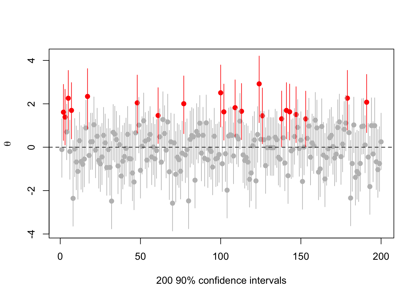
There are 21 intervals that miss zero, consistent with expectations. But they’re all centered at positive \(\theta\).
What happens if we vary the true \(\theta\)? Try \(\theta=1\) (now the red intervals are those that don’t cover 1)
set.seed(2019-6-11)
s<-make.s(1,1,1,.1)
rr<-replicate(200,{a<-rnorm(1,1);c(a,ci(a,1, s, 0.1))})
cover<-(rr[2,]<1) & (rr[3,]>1)
plot(1:200, rr[1,],ylim=range(rr),pch=19,col=ifelse(cover,"grey","red"),
ylab=expression(theta),xlab="200 90% confidence intervals")
segments(1:200,y0=rr[2,],y1=rr[3,],col=ifelse(cover,"grey","red"))
abline(h=1,lty=2)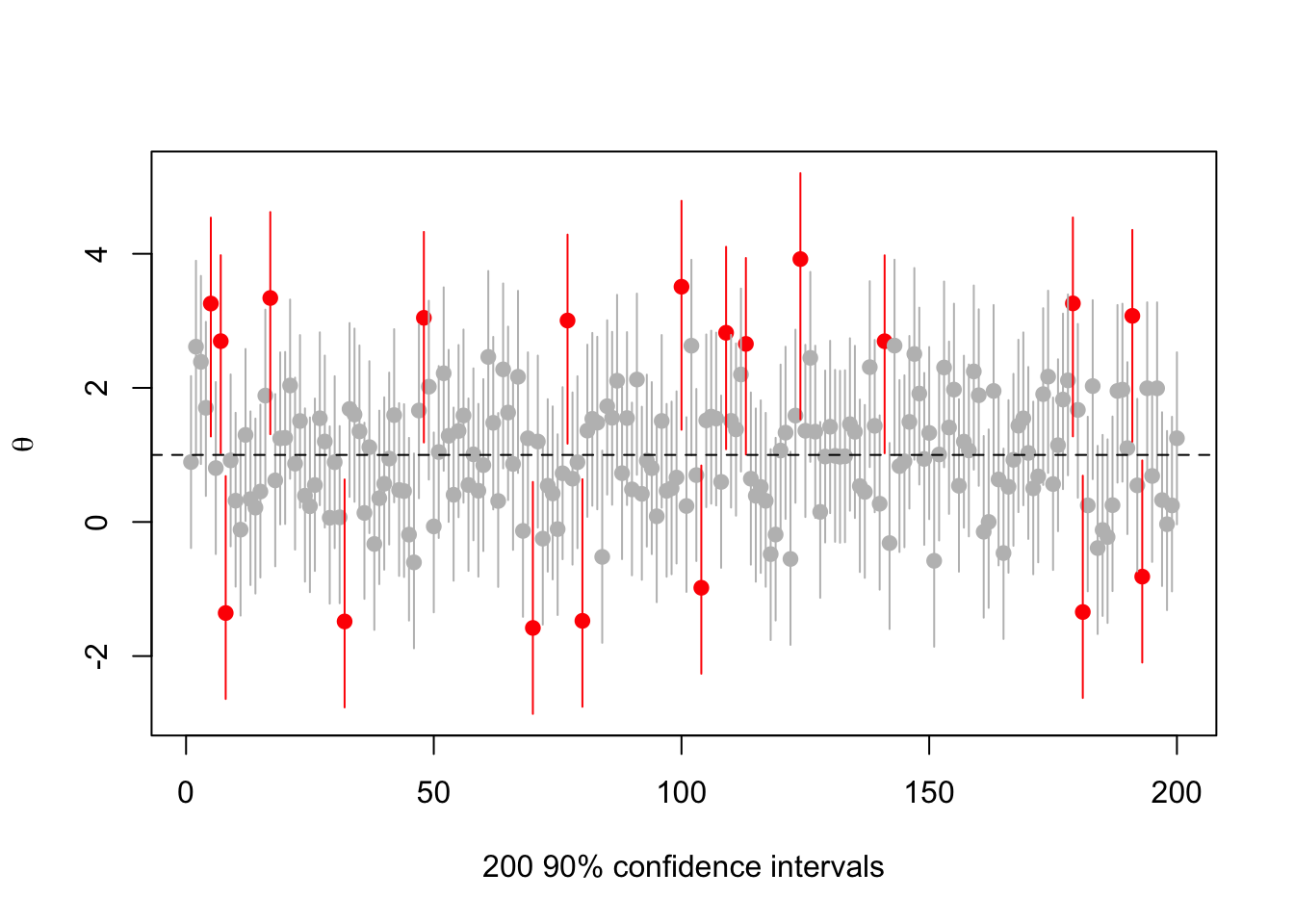
Or \(\theta=2\)
set.seed(2019-6-11)
s<-make.s(1,1,1,.1)
rr<-replicate(200,{a<-rnorm(1,2);c(a,ci(a,1, s, 0.1))})
cover<-(rr[2,]<2) & (rr[3,]>2)
plot(1:200, rr[1,],ylim=range(rr),pch=19,col=ifelse(cover,"grey","red"),
ylab=expression(theta),xlab="200 90% confidence intervals")
segments(1:200,y0=rr[2,],y1=rr[3,],col=ifelse(cover,"grey","red"))
abline(h=2,lty=2)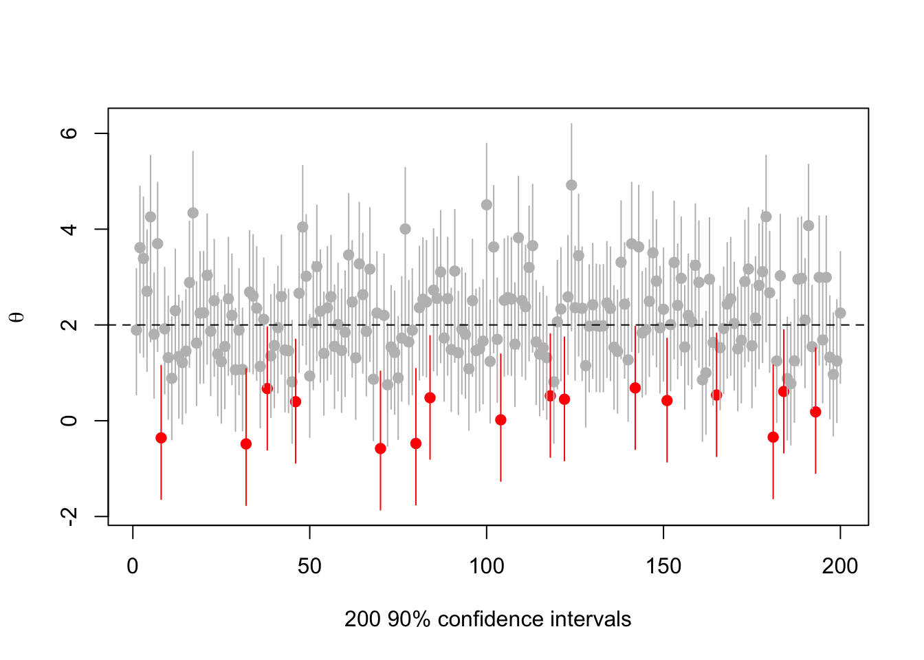
Or \(\theta=-1\)
set.seed(2019-6-11)
s<-make.s(1,1,1,.1)
rr<-replicate(200,{a<-rnorm(1,-1);c(a,ci(a,1, s, 0.1))})
cover<-(rr[2,]< -1) & (rr[3,]> -1)
plot(1:200, rr[1,],ylim=range(rr),pch=19,col=ifelse(cover,"grey","red"),
ylab=expression(theta),xlab="200 90% confidence intervals")
segments(1:200,y0=rr[2,],y1=rr[3,],col=ifelse(cover,"grey","red"))
abline(h=-1,lty=2)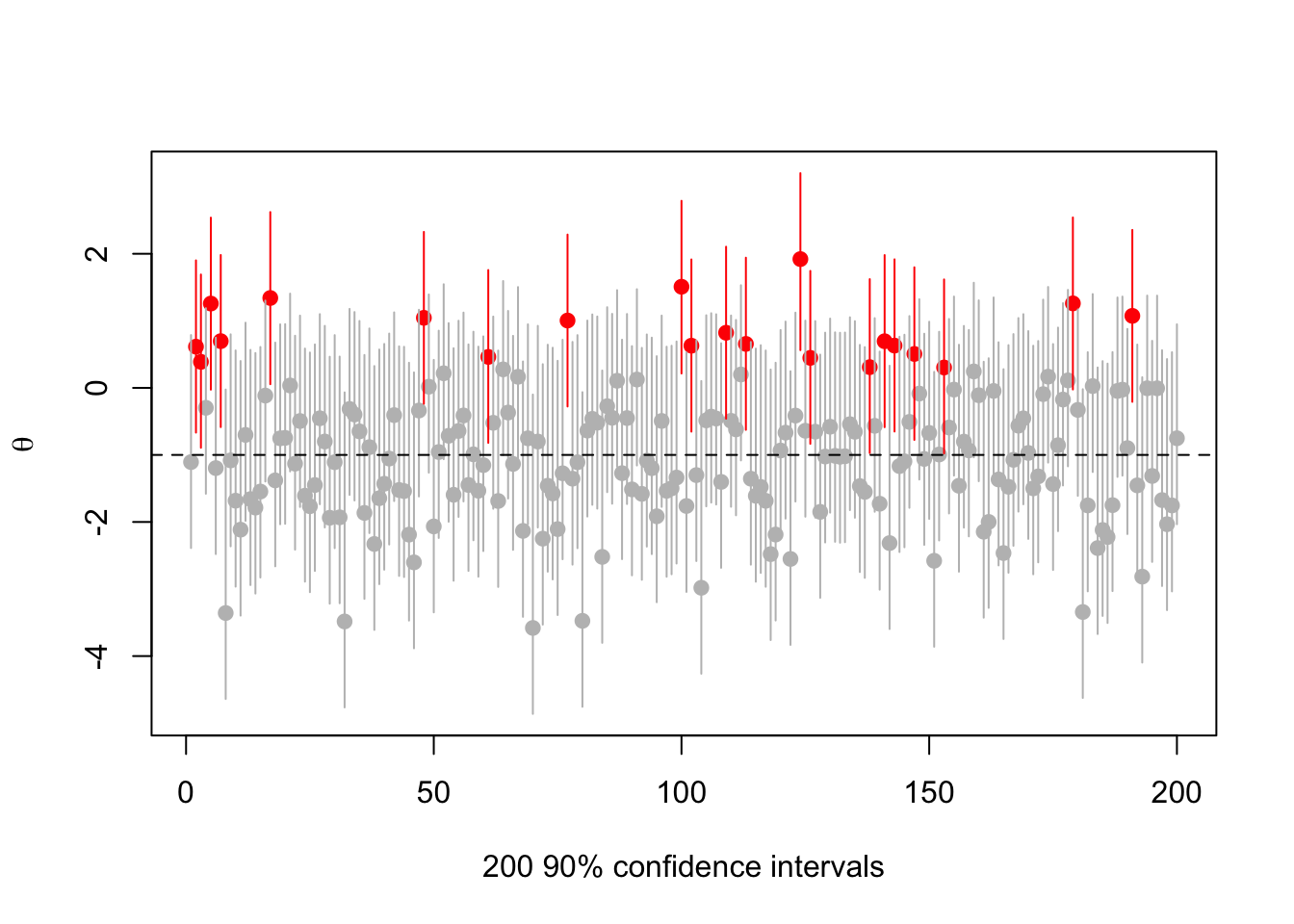
There’s nothing actually wrong here, but it’s messing with people’s natural misunderstandings of confidence intervals in order to push the impression that \(\theta\approx 1\).
I think I like it. Or maybe I don’t. One or the other.