Confidence intervals: not a very strong property

It’s important for non-Bayesians (or non-exclusively-Bayesians) to remember that being a 95% confidence interval procedure is a fairly weak property. It’s not that confidence intervals are necessarily bad, but if they aren’t, it’s because of other requirements.

As an extreme case, consider the all-purpose data-free exact confidence interval procedure for any real quantity: roll a d20 and set the confidence interval to be the empty set if you roll 20, and otherwise to be $R$. That’s a valid confidence interval procedure, it’s just a stupid one.

A much more interesting example comes from a recent paper by Kyle Burris and Peter Hoff, in the context of small-area sampling. First, suppose you have a random variable $y\sim N(\theta ,{\sigma }^2)$ with ${\sigma }^2$ known. They say “it is easily verified that” for any function $s:R\to [0,1]$, $$C_s=\{\theta :y+\sigma z_{\alpha (1-s(\theta \left)\right)}<\theta <y+\sigma z_{1-\alpha s\left(\theta \right)}\}$$ defines a $1-\alpha$ confidence interval. If you stare at this for a while, you seee that you’re doing a level-$\alpha$ test at each value of $\theta$, but that $s\left(\theta \right)$ tells you how to split $\alpha$ between upper and lower tails. With $s\left(\theta \right)=1/2$ you get the standard equal-side test; with $s\left(\theta \right)=0$ you get the lower side only; with $s\left(\theta \right)=1$ you get the upper side only.

What’s unusual is that you get to choose $s\left(\theta \right)$ separately for each $\theta$. That’s fine from the formal definition of confidence intervals: the $1-\alpha$ coverage property only needs to hold for the true $\theta$, so we need only consider one $\theta$ at a time. But it’s a bit weird.

In the small-area sampling context you have lots of $\theta$s, $y$s, $\sigma$s, and so on, one for each small area, and you get sets of intervals $$C_s^j=\{\theta :y_j+{\sigma }_j{z}_{\alpha (1-s_j(\theta \left)\right)}<\theta <y_j+{\sigma }_j{z}_{1-\alpha s_j\left(\theta \right)}\}$$

From a sampling/frequency point of view, the true ${\theta }_j$ are fixed, and $y_j-{\theta }_j$ depends only on sampling variability. So it’s perfectly ok to allow $s_j\left(\theta \right)$ to depend on data from areas other than area $j$.

In particular, you might have a prior for ${\theta }_j$ based on the data from all the other areas, say ${\theta }_j\sim N({\mu }_j,{\tau }_j^2)$, and you might want to have shorter confidence intervals when ${\theta }_j$ is near ${\mu }_j$. You can do this by biasing the two-sided test to reject on the lower side for ${\theta }_j<{\mu }_j$ and on the upper side for ${\theta }_j>{\mu }_j$. Specifically, Burris & Hoff define $$g\left(\omega \right)={\Phi }^{-1}\left(\alpha \omega \right)-{\Phi }^{-1}\left(\alpha \right(1-\omega \left)\right)$$ and then $$s_j\left(\theta \right)=g^{-1}\left(2{\sigma }_j\right(\theta -{\mu }_j\left)/ta{u}_j^2\right)$$ and show this all works, and something similar works in the more-plausible setting where you don’t know the $\sigma$s.

In R

make.s<-function(mu, sigma,tau2,alpha){
    g<-make.g(alpha)
    ginv<-make.ginv(alpha)
    
    function(theta) ginv(2*sigma*(theta-mu)/tau2)
}

make.g<-function(alpha){
    function(omega) qnorm(alpha*omega)-qnorm(alpha*(1-omega))
}
make.ginv<-function(alpha){
    g<-function(omega)  qnorm(alpha*omega)-qnorm(alpha*(1-omega))
    function(x){
        f<-function(omega) g(omega)-x
        if (x<0) {
            uniroot(f,c(pnorm(x/alpha),0.5))$root
        } else if (x==0) {
            0.5
        } else 
            uniroot(f,c(0.5,pnorm(x/alpha)))$root
    }
}

ci<-function(y, sigma, s,alpha){

    f_low<-function(theta) theta-(y+sigma*qnorm(alpha*(1-s(theta))))
    f_up<-function(theta) (y+sigma*qnorm(1-alpha*s(theta)))-theta

    low0<-y+qnorm(alpha/2)*sigma
    low1<-low0
    low<-if (f_low(low1)>0){
        while(f_low(low1)>0) low1<- y+(low1-y)*2
        uniroot(f_low,c(low1,low0))$root
    } else{
        uniroot(f_low,c(low0,y))$root
    }
    hi0<-y+qnorm(1-alpha/2)*sigma
    hi1<-hi0
    high<-if (f_up(hi1)>0){
        while(f_up(hi1)>0) hi1<- y+(hi1-y)*2
        uniroot(f_up,c(hi0,hi1))$root
    } else{
        uniroot(f_up,c(y,hi0))$root
    }
    
    c(low,high)
}

There’s a sense in which this has got to be cheating. In some handwavy sense, you’re sort of getting away with a $1-2\alpha$ confidence interval near ${\mu }_j$ at the expense of overcoverage elsewhere. But not really. The intervals really have $1-\alpha$ coverage: if you generated data for any true $\theta$ and used this procedure, $1-\alpha$ of the intervals would cover that true $\theta$, whatever it was. It’s all good.

But there’s nothing in the maths that requires ${\mu }_j$ to be a prior mean. It could also be that ${\mu }_j$ is the value you want to convince people that ${\theta }_j$ has. Again, you’ll get shorter confidence intervals when they’re centered near your preferred value and longer ones when they aren’t; again, they’ll have $1-\alpha$ coverage

Here’s an example with the true $\theta =0$, with $\sigma =1$, $\mu =1$, $\tau =1$, and with $\alpha =0.1$ to make it easier to see. So, we’d like to convince people that $\theta \approx 1$, but we aren’t allowed to mess with the 90% confidence level

set.seed(2019-6-11)
s<-make.s(1,1,1,.1)
rr<-replicate(200,{a<-rnorm(1);c(a,ci(a,1, s, 0.1))})
cover<-(rr[2,]<0) & (rr[3,]>0)
plot(1:200, rr[1,],ylim=range(rr),pch=19,col=ifelse(cover,"grey","red"),
ylab=expression(theta),xlab="200 90% confidence intervals")
segments(1:200,y0=rr[2,],y1=rr[3,],col=ifelse(cover,"grey","red"))
abline(h=0,lty=2)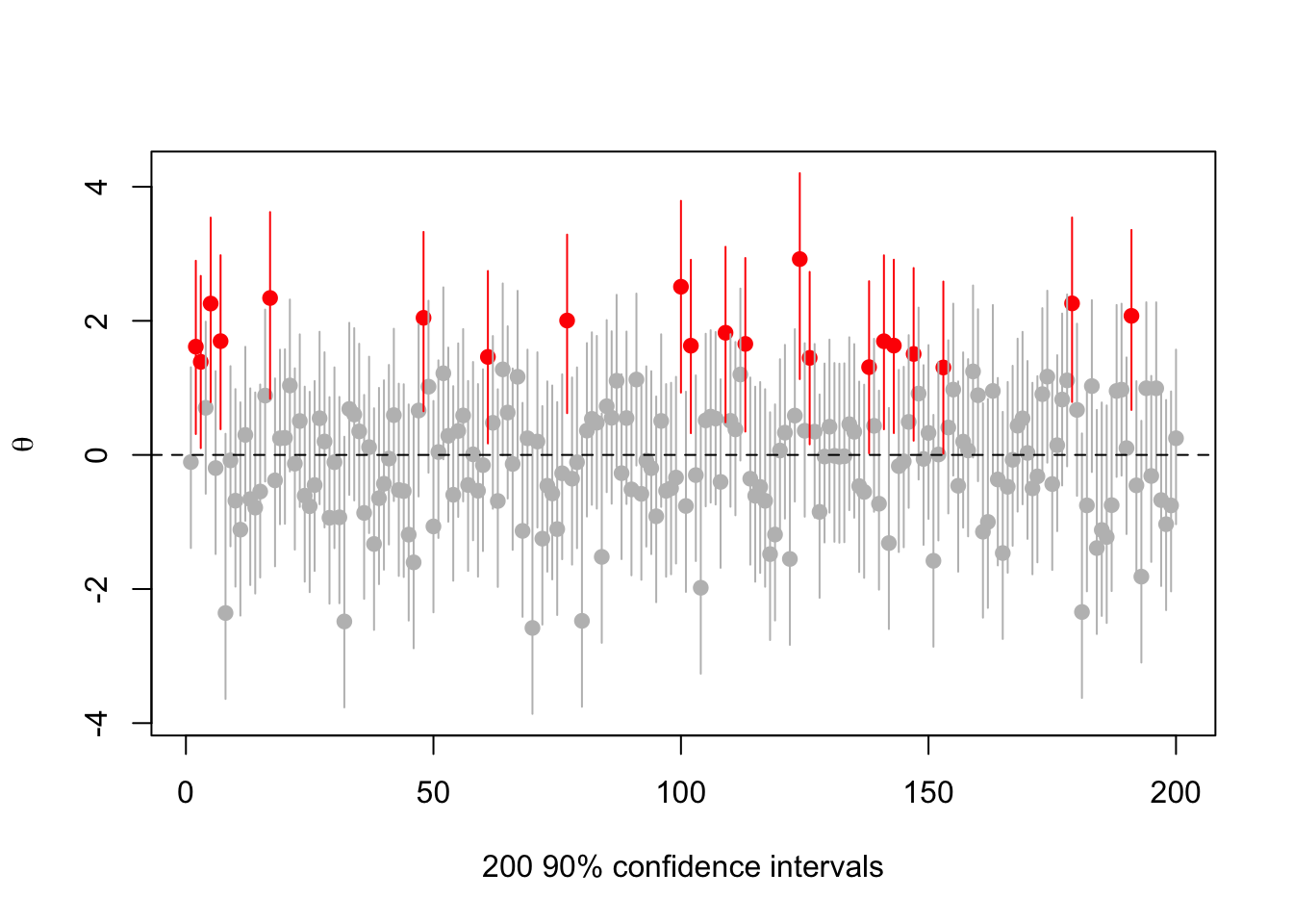

There are 21 intervals that miss zero, consistent with expectations. But they’re all centered at positive $\theta$.

What happens if we vary the true $\theta$? Try $\theta =1$ (now the red intervals are those that don’t cover 1)

set.seed(2019-6-11)
s<-make.s(1,1,1,.1)
rr<-replicate(200,{a<-rnorm(1,1);c(a,ci(a,1, s, 0.1))})
cover<-(rr[2,]<1) & (rr[3,]>1)
plot(1:200, rr[1,],ylim=range(rr),pch=19,col=ifelse(cover,"grey","red"),
ylab=expression(theta),xlab="200 90% confidence intervals")
segments(1:200,y0=rr[2,],y1=rr[3,],col=ifelse(cover,"grey","red"))
abline(h=1,lty=2)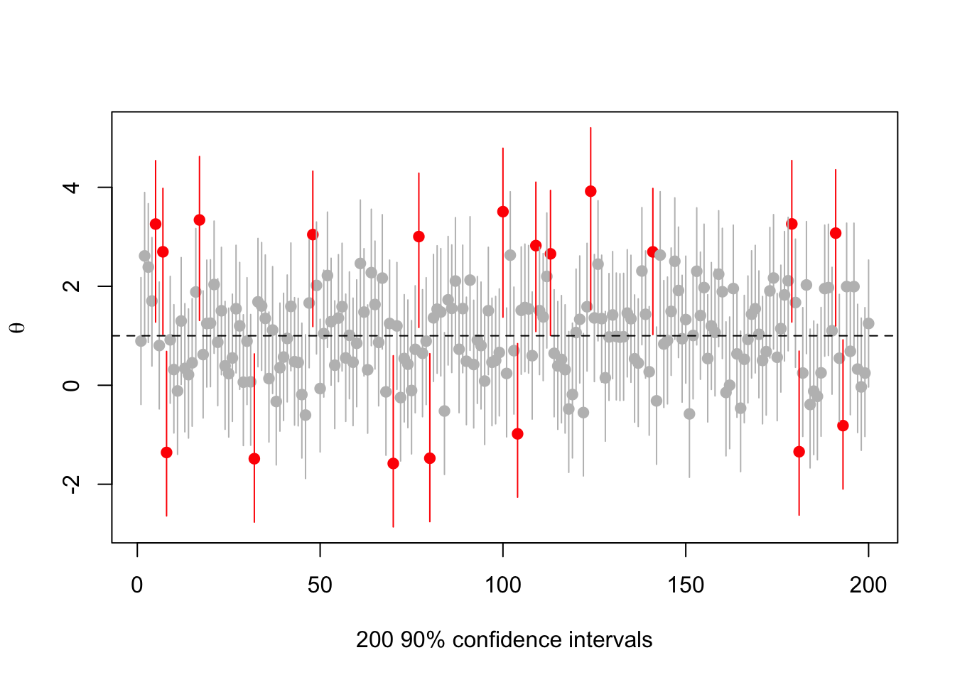

Or $\theta =2$

set.seed(2019-6-11)
s<-make.s(1,1,1,.1)
rr<-replicate(200,{a<-rnorm(1,2);c(a,ci(a,1, s, 0.1))})
cover<-(rr[2,]<2) & (rr[3,]>2)
plot(1:200, rr[1,],ylim=range(rr),pch=19,col=ifelse(cover,"grey","red"),
ylab=expression(theta),xlab="200 90% confidence intervals")
segments(1:200,y0=rr[2,],y1=rr[3,],col=ifelse(cover,"grey","red"))
abline(h=2,lty=2)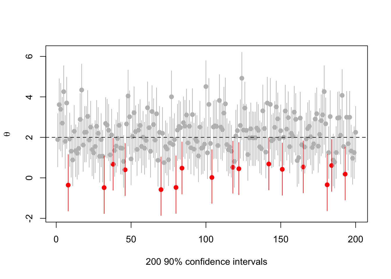

Or $\theta =-1$

set.seed(2019-6-11)
s<-make.s(1,1,1,.1)
rr<-replicate(200,{a<-rnorm(1,-1);c(a,ci(a,1, s, 0.1))})
cover<-(rr[2,]< -1) & (rr[3,]> -1)
plot(1:200, rr[1,],ylim=range(rr),pch=19,col=ifelse(cover,"grey","red"),
ylab=expression(theta),xlab="200 90% confidence intervals")
segments(1:200,y0=rr[2,],y1=rr[3,],col=ifelse(cover,"grey","red"))
abline(h=-1,lty=2)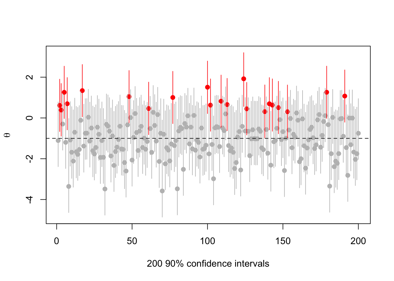

There’s nothing actually wrong here, but it’s messing with people’s natural misunderstandings of confidence intervals in order to push the impression that $\theta \approx 1$.

I think I like it. Or maybe I don’t. One or the other.