‘Network meta-analysis’ is the only term I’ve coined that’s actually entered the general biostatistical vocabulary. In network meta-analysis we work with a network of randomised trials, where the nodes are interventions and the edges are trials. A single edge represents a direct randomised comparison; a path represents an indirect (but unconfounded) estimate from multiple trials; we can combine multiple paths between interventions using a linear model.
For example, if \(\log RR_{ij,j}\) is the log relative risk in the \(k\)th trial of treatments \(i\) and \(j\), and it has variance \(\sigma^2_{ij,k}\) \[\log RR_{ij,k} = \beta_i-\beta_j+\epsilon_{ij,k}\] where \(\epsilon_{ij,k}\sim N(0,\sigma^2_{ij,k})\).
Here’s an example network, of trials of antihypertensive treatments that reported some real clinical outcomes such as heart attack or stroke. It’s the network from this paper, with \(\alpha\)-blockers taken out. 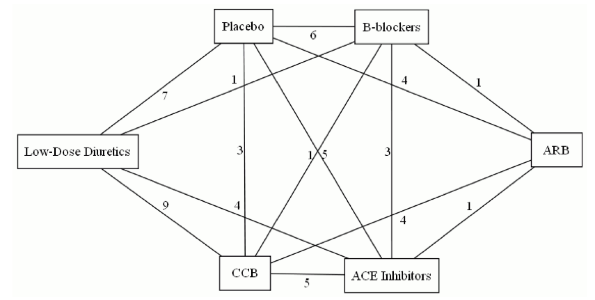
The simple linear model doesn’t allow for heterogeneity between trials of the same pair of treatments (heterogeneity), and also doesn’t allow for the effect of treatment \(i\) to be systematically different depending on what it’s compared two (which I called ‘incoherence’ and everyone else calls ‘inconsistency’). Heterogeneity and incoherence have the same basic causes: eg, differences in who would be randomised between this pair of treatments and in what other care they are given.
We know how to estimate heterogeneity for a given pair of treatments. Incoherence is only estimable when you have at least three treatments, and at least one loop in the network; one way to estimate it is by the sums of treatment effects around loops, which should be zero. We can fit a linear mixed model \[\log RR_{ij,k} = \beta_i-\beta_j+\epsilon_{ij,k}+\eta_{ij,k}+\xi_{ij}\] where now \(\eta\sim N(0,\tau^2_{ij})\) represents heterogeneity and \(\xi_{ij}\sim N(0,\omega^2)\) represents incoherence. Note that the incoherence effects \(\xi\) do not average away as \(k\) increases: they represent systematic differences in the sort of patients who were randomised between, say \(A\) vs placebo and \(A\) vs \(B\). The benefit of having a separate variance component for incoherence is that there’s not much information about incoherence in a typical network and we would prefer not to have it swamped by heterogeneity.
There’s a problem, though. The network above contains two three-armed trials. In a three-armed trial there is loop in the network entirely contained in one trial, which – as a matter of arithmetic – sums to zero. We will tend to underestimate incoherence when there are multi-armed trials. [Also, in a \(k\)-armed trial, each individuals contributes to \(k-1\) edges, but that can be handled by weighting]
The problem is because a graph is not a flexible enough data structure to represent multi-armed trials: we need a hypergraph. Hypergraphs sound scary, but there’s a straightforward representation of them as bipartite graphs: graphs with two types of nodes.
Here’s a simpler network: 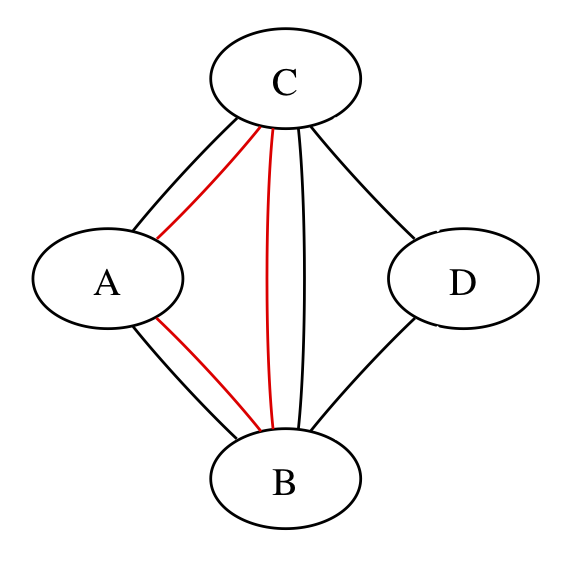
The three red edges could be three separate trials or three arms of one trial; the graph can’t distinguish, but the calculations have to.
We can rewrite the network with two sets of nodes – intervention nodes and trial nodes – and edges representing trial arms. If the three red edges are in different trials we get 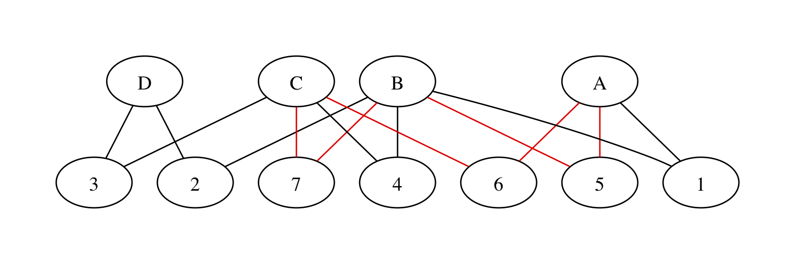
with trials numbered at random. We have all the same paths between treatments as in the original graph, but now a path between two treatments involves one or more pairs of edges. The edges in each pair must be necessarily be in the same trial or they won’t join up, so we’re still preserving randomisation. There’s still a red loop, as there should be: the red edges do contribute to incoherence.
If the three red edges are in the same trial, we get 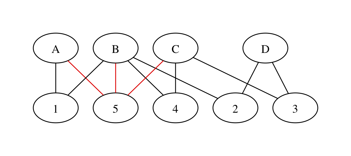
with no red loops. The spurious loop that’s entirely within the three-armed trial has disappeared!
We can now write a linear mixed model based on the bipartite graph. It’s harder to distinguish incoherence and heterogeneity. Writing \(P[\textrm{event}]_{i,k}\) for the probability of an event in trial \(k\), intervention \(i\), we could simplify to \[\log P[\textrm{event}]_{i,k} = \beta_i+\epsilon_{i,k}+\eta_{i,k}.\] To add incoherence we’d need \(\xi_{i:\textrm{combo}}\) random effects representing the bias in treatment \(i\) when it’s one of a specific combination of options. At that point it’s probably worth putting a more explicit prior on the incoherence effects.
Lin Bi did a short MSc research project with me on this idea, and it seems to work. Since that was in about 2012, it doesn’t look as though either of us is going to publish it any time soon, so at least there’s a blog post.