Survey analysis in SQL - Biased and Inefficient

Charco Hui, as his Honours project in Statistics, has been writing a package for complex-survey analysis using dplyr and dbplyr. It’s here. At the moment it has only been tested with MonetDB, using the github version (0.5.2) of MonetDBlite, but it should work with many other databases (not SQLite, at the moment). I hope it’s still under development: the approach does seem to be useful for large survey data sets – and for smaller data sets the dplyr version is faster than the survey package, though more limited.

Mostly, the package does the same things as my old sqlsurvey package, just with dbplyr as middleware to avoid hand-coding all the SQL. One newish thing is the code for hexagonal binning. In sqlsurvey I did this by reading the data into memory in chunks, but that’s not necessary.

The algorithm for hexagonal binning isn’t new: you compute which bin the point would go into for two offset rectangular grids and take the closer of the two resulting bin centres as the centre of the hex.

Here’s a simplified version in R, bypassing the trivial but annoying centering and scaling you need to get away from \((0,\,0)\), and not being quite careful enough about edge effects for outliers.

x<-rnorm(1000, sd=1)
y<-rnorm(1000, sd=sqrt(3))
x1<-round(x)
x2<-round(x+1/2)-1/2
y1<-round(y/sqrt(3))*sqrt(3)
y2<-(round(y/sqrt(3)+1/2)-1/2)*sqrt(3)
d1<-(x-x1)^2+3*(y-y1)^2
d2<-(x-x2)^2+3*(y-y2)^2
hx<-ifelse(d1<d2,x1,x2)
hy<-ifelse(d1<d2,y1,y2)
par(pty="s")
plot(x1,y1,pch=19)
points(x2,y2,pch=19,col="blue")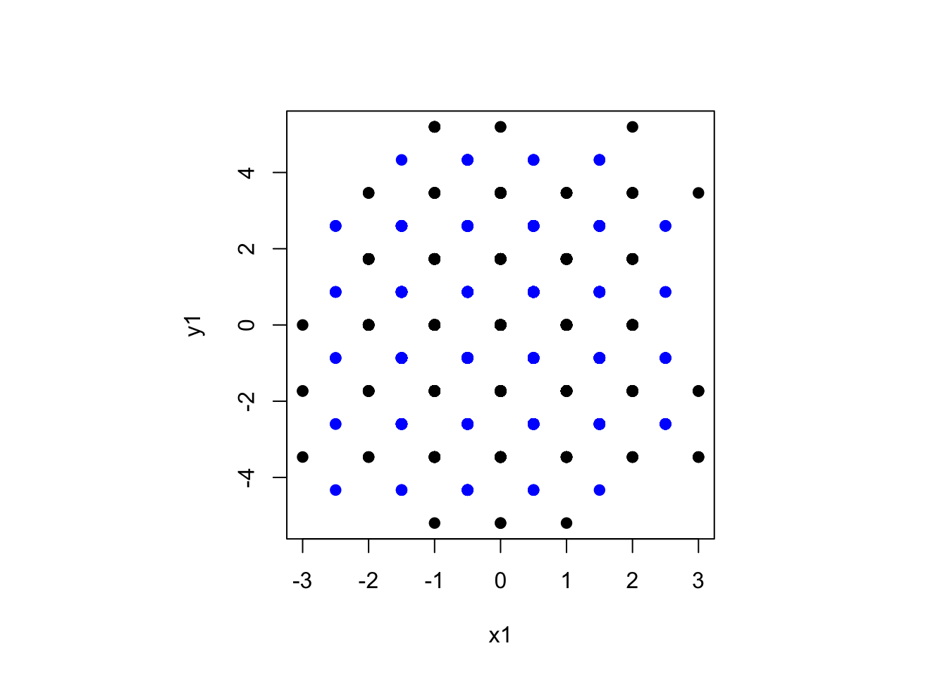

## now show how each point maps to a center
plot(hx,hy, col="#A000A020",pch=19)
points(x,y,pch=".")
segments(x,y,hx,hy,col="#00000060")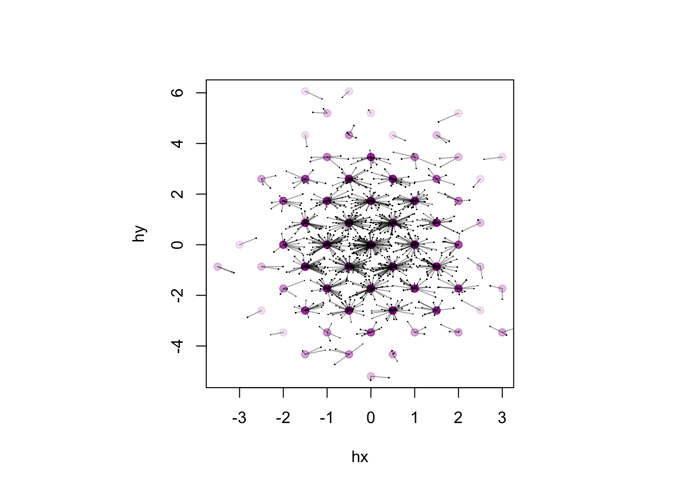

You can do this in dplyr, of course. This code doesn’t plot, but it shows the aggregation of points to hexes that you’d need for plotting

library(dplyr, quietly=TRUE)
tibble(x,y) %>% 
   mutate(x1=round(x),y1=round(y/sqrt(3))*sqrt(3), 
   x2=round(x+1/2)-1/2, y2=(round(y/sqrt(3)+1/2)-1/2)*sqrt(3)) %>%
   mutate(d1=(x-x1)^2+3*(y-y1)^2, d2=(x-x2)^2+3*(y-y2)^2) %>%
   mutate(hx=if_else(d1<d2,x1,x2), hy=if_else(d1<d2,y1,y2)) %>%
   group_by(hx,hy) %>% summarise(count=n())

## # A tibble: 65 x 3
## # Groups:   hx [?]
##       hx     hy count
##    <dbl>  <dbl> <int>
##  1  -3.5 -0.866     2
##  2  -3    0         1
##  3  -2.5 -2.60      1
##  4  -2.5 -0.866     2
##  5  -2.5  2.60      3
##  6  -2   -3.46      1
##  7  -2   -1.73      4
##  8  -2    0        12
##  9  -2    1.73      9
## 10  -1.5 -4.33      3
## # ... with 55 more rows

And once you’ve got in dplyr, you can just run it in dbplyr to do the computations in the database

For survey data, we want summarise(count=sum(weights)) rather than summarise(count=n()) so that the hex size depends on the estimated population size rather than the sample size, but otherwise it’s the same. That actually simplifies the edge-effect problem, as you can just add a point with zero weight at each potential hex center.

And here’s a small example,

# devtools:::install_github(chrk623/svydb)
library(svydb,quietly=TRUE)
library(DBI)
library(MonetDBLite)
con = dbConnect(MonetDBLite())

data(nhane)
dbWriteTable(con, "nhanes",nhane)

## Identifier(s) "X", "SurveyYr", "ID", "Gender", "Age", "AgeMonths", "Race1", "Race3", "Education", "MaritalStatus", "HHIncome", "HHIncomeMid", "Poverty", "HomeRooms", "HomeOwn", "Work", "Weight", "Length", "HeadCirc", "Height", "BMI", "BMICatUnder20yrs", "BMI_WHO", "Pulse", "BPSysAve", "BPDiaAve", "BPSys1", "BPDia1", "BPSys2", "BPDia2", "BPSys3", "BPDia3", "Testosterone", "DirectChol", "TotChol", "UrineVol1", "UrineFlow1", "UrineVol2", "UrineFlow2", "Diabetes", "DiabetesAge", "HealthGen", "DaysPhysHlthBad", "DaysMentHlthBad", "LittleInterest", "Depressed", "nPregnancies", "nBabies", "Age1stBaby", "SleepHrsNight", "SleepTrouble", "PhysActive", "PhyActiveDays", "TVHrsDay", "ComputerHrsDay", "Alcohol12PlusYr", "AlcoholDay", "AlcoholYear", "SmokeNow", "Smoke100", "SmokeAge", "Marijuana", "AgeFirstMarij", "RegularMarij", "AgeRegMarij", "HardDrugs", "SexEver", "SexAge", "SexNumPartnLife", "SexNumPartYear", "SameSex", "SexOrientation", "WTINT2YR", "WTMEC2YR", "SDMVPSU", "SDMVSTRA" contain uppercase or reserved SQL characters and need(s) to be quoted in queries.

## Identifier(s) "Work" are reserved SQL keywords and need(s) to be quoted in queries.

nhanes.db = tbl(con, "nhanes")
nh.dbsurv = svydbdesign(st = SDMVSTRA , wt = WTMEC2YR,id = SDMVPSU , data = nhanes.db)
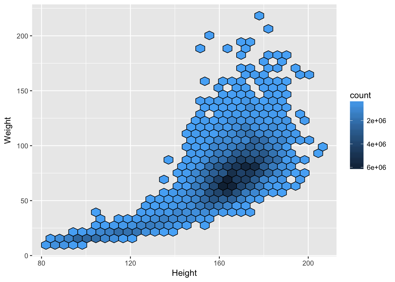
hb = svydbhexbin(Weight~Height , design = nh.dbsurv)
svydbhexplot(hb, xlab = "Height", ylab = "Weight")