If you know about design-based analysis of survey data, you probably know about the Rao-Scott tests, at least in contingency tables. The tests started off in the 1980s as “ok, people are going to keep doing Pearson \(X^2\) tests on estimated population tables, can we work out how to get \(p\)-values that aren’t ludicrous?” Subsequently, they turned out to have better operating characteristics than the Wald-type tests that were the obvious thing to do – mostly by accident. Finally, they’ve been adapted to regression models in general, and reinterpreted as tests in a marginal working model of independent sampling, where they are distinctive in that they weight different directions of departure from the null in a way that doesn’t depend on the sampling design.
The Rao–Scott test statistics are asymptotically equivalent to \((\hat\beta-\beta_0)^TV_0^{-1}(\hat\beta-\beta_0)\), where \(\hat\beta\) is the estimate of \(\beta_0\), and \(V_0\) is the variance matrix you’d get with full population data. The standard Wald tests are targetting \((\hat\beta-\beta_0)^TV^{-1}(\hat\beta-\beta_0)\), where \(V\) is the actual variance matrix of \(\hat\beta\). One reason the Rao–Scott score and likelihood ratio tests work better in small samples is just that score and likelihood ratio tests seem to work better in small samples than Wald tests. But there’s another reason.
The actual Wald-type test statistic (up to degree-of-freedom adjustments) is \((\hat\beta-\beta_0)^T\hat V^{-1}(\hat\beta-\beta_0)\). In small samples \(\hat V\) is often poorly estimated, and in particular its condition number is, on average, larger than the condition number of \(V\), so its inverse is wobblier. The Rao–Scott tests obviously can’t avoid this problem completely: \(\hat V\) must be involved somewhere. However, they use \(\hat V\) via the eigenvalues of \(\hat V_0^{-1}\hat V\); in the original Satterthwaite approximation, the mean and variance of these eigenvalues. In the typical survey settings, \(V_0\) is fairly well estimated, so inverting it isn’t a problem. The fact that \(\hat V\) is more ill-conditioned than \(V\) translates as fewer degrees of freedom for the Satterthwaite approximation, and so to a more conservative test. This conservative bias happens to cancel out a lot of the anticonservative bias and the tests work relatively well.
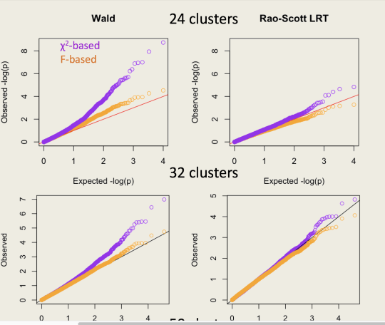
Here’s an example of qqplots of \(-\log_{10} p\)-values simulated in a Cox model: the Wald test is the top panel and the Rao–Scott LRT is the bottom panel. The clusters are of size 100; the orange tests use the design degrees of freedom minus the number of parameters as the denominator degrees of freedom in an \(F\) test.
So, what’s new? SUDAAN has tests they call “Satterthwaite Adjusted Wald Tests”, which are based on \((\hat\beta-\beta_0)^T\hat V_0^{-1} (\hat\beta-\beta_0)\). I’ve added similar tests to version 3.33 of the survey package (which I hope will be on CRAN soon). These new tests are (I think) asymptotically locally equivalent to the Rao–Scott LRT and score tests. I’d expect them to be slightly inferior in operating characteristics just based on traditional folklore about score and likelihood ratio tests being better. But you can do the simulations yourself and find out.
The implementation is in the regTermTest() function, and I’m calling these “working Wald tests” rather than “Satterthwaite adjusted”, because the important difference is the substitution of \(V_0\) for \(V\), and because I don’t even use the Satterthwaite approximation to the asymptotic distribution by default.