Attention Conservation Notice: Very long and involves a proof that hasn’t been published, though the paper was rejected for unrelated reasons.
Basically everything in statistics is a sum, and the basic useful fact about sums is the Law of Large Numbers: the sum is close to its expected value. Sometimes you need more, and there are lots of uses for a good bound on the probability of medium to large deviations from the expected value.
One of the nice ones is Bernstein’s Inequality, which applies to bounded variables. If the variables have mean zero, are bounded by \(\pm K\), and the variance of the sum is \(\sigma^2\), then
\[\Pr\left(\left|\sum_i X_i\right|>t\right)\leq 2e^{-\frac{1}{2}\frac{t^2}{\sigma^2+Kt}}.\]
The bound is exponential for large \(t\) and looks like a Normal distribution for small \(t\). You don’t actually need the boundedness; you just need the moment bounds it implies: for all \(r>2\), \(EX_i^r\leq K^{r-2}r!E[X_i^2]/2\). That looks like the Taylor series for the exponential, and indeed it is.
These inequalities tend to only hold for sums of independent variables, or ones that can be rewritten as independent, or nearly independent. My one, which this post is about, is for what I call sparse correlation. Suppose you’re trying to see how accurate radiologists are (or at least, how consistent they are). You line up a lot of radiologists and a lot of x-ray images, and get multiple ratings. Any two ratings of the same image will be correlated; any two ratings by the same radiologist will be correlated; but ‘most’ pairs of ratings will be independent.
You might have the nice tidy situation where every radiologist looks at every image, in which case you could probably use \(U\)-statistics to prove things about the analysis. More likely, though, you’d divide the images up somehow. For rating \(X_i\), I’ll write \({\cal S}_i\) as the set of ratings that aren’t independent of \(X_i\), and call it the neighbourhood of \(X_i\). You could imagine a graph where each observation has an edge to each other observation in its neighbourhood, and this graph will be important later.
I’ll write \(M\) for the size of the largest neighbourhood and \(m\) for the size of the largest set of independent observations. If you had 10 radiologists each reading 20 images, \(M\) would be \(10+20-1\) and \(m\) would be \(10\). I’ll call data sparsely correlated if \(Mm\) isn’t too big. If I was doing asymptotics I’d say \(Mm=O(n)\)
I actually need to make the stronger assumption that any two sets of observations that aren’t connected by any edges in the graph are independent: pairwise independence isn’t enough. For the radiology example that’s still fine: if set A and set B of ratings don’t involve any of the same images or any of the same radiologists they’re independent.
A simple case of sparsely correlated data that’s easy to think about (if pointless in the real world) is identical replicates. If we have \(m\) independent observations and take \(M\) copies of each one, we know what happens to the tail probabilities: you need to replace \(t\) by \(Mt\) and \(\sigma^2\) by \(M\sigma^2\) (ie, \(M^2\) times the sum of the \(m\) independent variances). We can’t hope to do better; it turns out we can do as well.
The way we get enough independence to use the Bernstein’s-inequality argument is to make up \(M-1\) imaginary sets of data. Each set has the same joint distribution as the original variables, but the sets are independent of each other. Actually, what we need is not \(M\) copies but \(\chi\) copies, where \(\chi\) is the number of colours needed for every variable in the dependency graph to have a different colour from all its neighbours. \(M\) is always enough, but you can sometimes get away with fewer.
Here’s the picture, for a popular graph
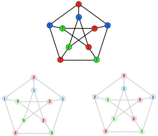
The original variables are at the top. We needed three colours, so we have the original variables and two independent copies.
Now look at the points numbered ‘1′. Within a graph these are never neighbours because they are the same colour, and obviously between graphs they can’t be neighbours. So, all the variables labelled `1′ are independent (even though they have horribly complicated relationships with variables of different labels). There’s a version of every variable labelled ‘1′, another version labelled ‘2′, and another labelled ‘3′.
The proof has five steps. First, we work with the exponential of the sum in order to later use Markov’s inequality to get exponential tail bounds. Second, we observe that adding all these extra copies makes the problem worse: a bound for the sum of all \(M\) copies will bound the original sum. Third, we use the independence within each label to partially factorise an expectation of \(e^{\textrm{sum}}\) into a product of expectations. We use the original Taylor-series argument based on the moment bounds to get a bound for an exponential moment. And, finally, we use Markov’s inequality to turn that into an exponential tail bound. The first, and last two, steps are standard, the second and third are new.
Theorem: Suppose we have \(X_i\), \(i=1,2,\ldots,n\) mean zero with neighbourhood size \(M\). Suppose that for each \(X_i\)
\[ EX_i^r\leq K^{r-2}r!\sigma_i^2/2\]
and let \(\sigma^2\geq\sum_{i=1}^n\sigma_i^2\)
Then
\[\Pr\left(\left|\sum_i X_i\right|>t\right)\leq2e^{-\frac{1}{2}\frac{t^2}{M\sigma^2+MKt}}.\]
Proof: The \(M\) copies of the variables are written \(\tilde X_{ij}\) with \(i=1,\dots,n\) and \(j=1,\dots,M\), and the labelled versions as \(X_{i(j)}\) for the copy of \(X_i\) labelled \(j\).
By independence of the copies from each other
\[\begin{eqnarray*}
E\left[\exp(\frac{1}{M}\sum_{j=1}^M\sum_{i=1}^n\tilde X_{ij}) \right]&=&\prod_{j=1}^ME\left[\exp(\frac{1}{M}\sum_{i=1}^n\tilde X_{ij}) \right]\\
&=&E\left[\exp(\frac{1}{M}\sum_{i=1}^nX_{i}) \right]^M\\\
&\geq&E\left[\exp(\frac{1}{M}\sum_{i=1}^nX_{i}) \right]
\end{eqnarray*}\]
so introducing the extra copies makes things worse.
Now we use the labels. We can factor the expectation into a product over \(i\), since \(X_{i(j)}\) with the same \(j\) and different \(i\) are independent.
\[E\left[\exp(\frac{1}{M}\sum_{j=1}^M\sum_{i=1}^n\tilde X_{i(j)}) \right]=\prod_i E\left[\exp\left(\frac{1}{M}\sum_{j=1}^M \tilde X_{i(j)} \right)\right]\]
Now we use the moment assumptions to get moment bounds for the sum
\[E\left[\left(\frac{1}{M}\sum_{j=1}^M\sum_{i=1}^n\tilde X_{i(j)}\right)^r\;\right]\leq M^{r-1}E\left[\left(\sum_{i=1}^n \tilde X_{i1}\right)^r\,\right]\leq M^{r-1}r!K^{r-2}\sigma^2\]
Writing \(S_n\) for \(\sum_{i=1}^n X_i\), and \(\tilde S_n\) for \(\sum_{i,j} \tilde X_{ij}\) we have (for a value \(c\) to be chosen later)
\[\begin{eqnarray*}
E e^{cS_n} &\leq& Ee^{c\tilde S_n}\\
&=& 1+\frac{1}{2}\sigma^2c^2\sum_{r=2}^\infty \frac{c^{r-2}E\tilde S_n^r}{r!\sigma^2/2}\\
&<&\exp\left[\frac{1}{2}\sigma^2c^2\sum_{r=2}^\infty \frac{c^{r-2}E\tilde S_n^r}{r!\sigma^2/2}\right]\\
&\leq&\exp\left[\frac{1}{2}\sigma^2c^2\sum_{r=2}^\infty \frac{c^{r-2}M^{r-1}r!K^{n-2}\sigma^2/2}{r!\sigma^2/2}\right]\\
&<&\exp\left[\frac{1}{2}M\sigma^2c^2\sum_{r=2}^\infty(cMK)^{r-2} \right]\\
&=&\exp\left[\frac{M\sigma^2c^2}{2(1-cMK)}\right]
\end{eqnarray*}\]
Write \(\tilde K\) for \(MK\) and \(\tilde \sigma^2\) for \(M\sigma^2\) to get
\[E e^{cS_n}<\exp\left[\frac{\tilde\sigma^2c^2}{2(1-c\tilde K)}\right]\]
Markov’s inequality now says
\[P[S_n\geq t\tilde\sigma]\leq \frac{Ee^{cS_n}}{e^{ct\tilde\sigma}}<\exp\left[\frac{\tilde\sigma^2c^2}{2(1-c\tilde K)}-ct\tilde\sigma\right],\]
We’re basically done: we just need to find a good choice of \(c\). The calculations are the same as in Bennett’s 1962 proof of Bernstein’s inequality, where he shows that \(c=t/(\tilde Kt+\tilde \sigma)\) gives
\[P[S_n\geq t]<\exp\left[-\frac{1}{2}\frac{t^2}{\tilde\sigma^2+\tilde Kt}\right]\]
That’s an upper bound, and adding the same lower bound at most doubles the tail probability. So we are done.