The basic story about sampling weights and regression is fairly simple: if you don’t need the weights, using them will add noise. The standard error increase is basically proportional to the coefficient of variation of the weights, and doesn’t depend on the regression coefficients or the covariate distribution.
Logistic regression in a case-control sample looks superficially as if it should be the same. The maximum likelihood estimator is unweighted logistic regression, ignoring the weights, and it’s more efficient that the estimator using sampling weights. But logistic regression is different: the sampling isn’t actually non-informative, it’s just that all the bias magically ends up in the intercept, which we don’t usually care about. The efficiency gap is different, too.
This graph shows the ratio of the standard errors for a model \(\mathrm{logit}\,\Pr[Y=1]=\alpha+X\), with \(X\sim N(0,1)\) and various numbers of controls per case. In each simulation, \(\alpha\) is chosen so the control sampling fraction is the same (1%), so the coefficient of variation of the weights is the same everywhere. The efficiency loss isn’t, to put it mildly

As another example, consider a variable with values 1-4. This graph shows control distributions in black and the implied case distributions for \(\beta=1\) in red.

And here are the standard error ratios
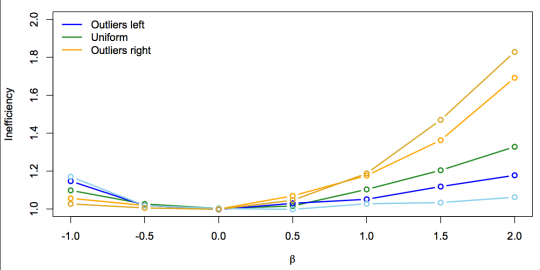
An explanation that predicts these results (it honestly was a prior prediction, though not preregistered), is based on multiple imputation. Suppose we didn’t know what the maximum likelihood estimator was, but we were prepared to do multiple imputation of \(X\) for all the unobserved non-cases. If we do this right and all the assumptions hold and so on, it should recover the maximum likelihood estimator. There’s information about the non-case distribution of \(X\) in controls, obviously. There’s also information in the cases: the density of \(X\) in cases is proportional to the density in controls scaled by \(e^{\beta x}\). If we impute using only the control distribution we just get the weighted estimator, so the efficiency gap must be explained by the information in cases about the control \(X\) distribution.
So, one way to predict whether the gain in precision is large or small is to see if the case \(X\) distribution contains large or small amounts of information about the control \(X\) distribution: are there lots of cases at \(X\) values with few controls?
The bar plots suggest that for positive \(\beta\) and positively-skewed \(X\) there should be a large gain, but it should be smaller for uniform or negatively skewed \(X\), and the pattern should reverse for negative \(\beta\). As it does. Also, as the number of controls increases, the extra information from the cases will become less important, so the efficiency gap will decrease. As it does.
This has been another episode of Case-control logistic regression is more complicated than you think. It’s going to be a talk in Auckland on April 5 and at U Penn on April 20.