So, I have been asked a few times how to compute \(R^2\) for models fitted to survey data. Initially the questions were about the ordinary linear-regression \(R^2\), which is easy because it’s the ratio of two variances, and we can estimate variances. More recently, people have been asking about the Nagelkerke pseudo-\(R^2\) in logistic regression.
It’s not immediately obvious how to define the Nagelkerke \(R^2\) under complex sampling. My approach was to consider the Cox–Snell \(R^2\) that precedes it, which is an estimate of a well-defined population quantity: \(\log (1-R^2)\) is the mutual information between the predictors and outcome. Replacing the likelihood in the definitions by the estimated population likelihood gives a design-based definition of the Cox–Snell \(R^2\), and the Nagelkerke \(R^2\) is a simple rescaling. I’ve got a preprint here and code here. [Update: the paper is out, at ANZ J Stat]
With any design-based statistic for logistic regression it’s natural to look at case–control designs as an example. These have highly informative sampling, so that ignoring the sampling weights will lead to bias. Usually we don’t worry about the bias, because in a logistic regression model it’s all in the intercept, and not in the other regression parameters. However, when you have a statistic that isn’t just a function of the regression slopes, you have to worry about whether the bias reappears.
It does.
The following picture shows a series of simulated case-control designs with \(X\sim N(0,1)\), \(\textrm{logit}\,P[Y=1]=-6+x\), and 1,2,5,10, or 20 controls per case. The three lines are the ordinary Nagelkerke \(R^2\), Cox–Snell \(R^2\), and a trendy new one due to Tjur. The x-axis gives the control sampling percentage, and the horizontal dashed lines are the \(R^2\) values for a model fitted to the full cohort.
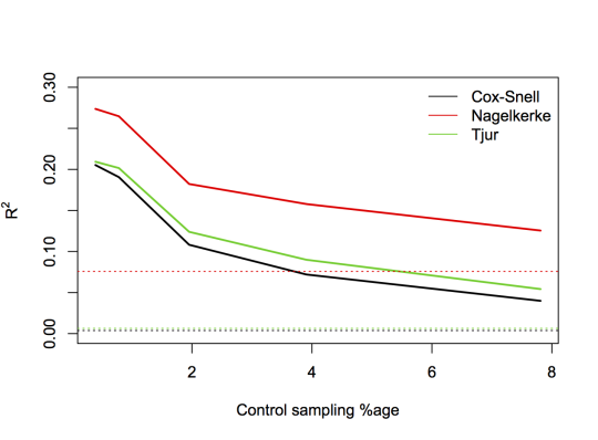
As you can see, there’s a lot of bias. Under case–control sampling, the standard forms of all three of these \(R^2\) statistics are inflated relative to the value you would get with full-cohort data.
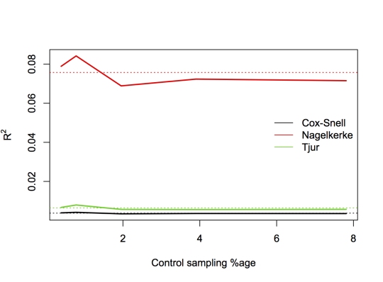
While I could imagine someone coming up with a reason to prefer the in-sample \(R^2\) rather than the full-cohort one, the usual motivation for case-control sampling is to estimate the properties of the cohort and the population from which it comes, not properties of the sample. So, design-based versions of these statistics should be useful. My preprint shows how to define and compute design-based versions of Nagelkerke and Cox–Snell statistics. The Tjur statistic is easy: it’s the mean of \(\\hat Y\) in cases minus the mean in non-cases, so a design-based version just needs weighted means.
As evidence that the deisgn-based versions work, here’s the same sequence of designs with survey-weighted models and design-based \(R^2\) statistics:
I was surprised that Cox and Snell didn’t notice and comment on this phenomenon, but on looking up the reference I found it’s an exercise in their book Analysis of Binary Data