Attention Conservation Notice: there probably aren’t as many as half a dozen groups in the world who actually have this much genome sequencing data. Everyone else could wait to see if something better comes up.
If you follow me on Twitter, you will have seen various comments about eigenvalues, matrices, and other linear algebra over the past months. Here, finally, is the Sekrit Eigenvalue Project.
A quadratic form in Normally distributed variables is of the form \(z^TAz\) where \(z\) is a vector of \(n\) standard Normals and \(A\) is an \(n\times n\) matrix. Obviously the \(z\)s might not be independent or unit variance; almost equally obviously you can fix that by changing \(A\). If \(A\) is (a multiple of) a projection matrix of rank \(p\), the distribution is (a multiple of) \(\chi^2_p\), but not otherwise.
These quadratic forms come up naturally in two settings in statistics. The first is misspecified likelihood ratio tests. If you do a second-order Taylor series expansion of the difference in log likelihoods you find that the linear term vanishes because you’re at the maximum, and the quadratic term annoyingly fails to collapse into the \(\chi^2_p\) of correctly-specified nested models. The other setting is when you take a set of asymptotically Normal test statistics and profane the Gauss-Markov theorem by deliberately combining them with something other than their true inverse variance matrix as weights.
Two popular use cases for the latter setting are the Rao-Scott tests in survey statistics and the SKAT (sequence kernel association test) in genomics. In the Rao-Scott test the individual statistics are observed minus expected counts for cells in a table; in the SKAT test they are covariances between individual rare variants and phenotype. In both settings the true variance matrix of the individual statistics tends to be poorly estimated, so you do better by using something simpler: the Rao–Scott test uses the matrix that would be the variance under iid sampling, the SKAT test uses a set of weights that ignore correlation and upweight less-common variants.
The null distribution of the resulting test is a linear combination of \(\chi^2_1\) variables, where the coefficients in the linear combination are the eigenvalues of \(A\). That’s not in the tables in the back of the book, but there are several perfectly good ways of working it out given the eigenvalues.
In some genomic problems, though, the matrix \(A\) is big, with \(n\) easily being as much as several thousands now, and much larger in the future. Computing the eigenvalues takes time. Even computing the matrix \(A\) is not trivial – the time complexity of both tasks scales as the cube of sample size (or number of genetic variants). That is, the time complexity for computing the sampling distribution goes up faster than the data size, even though the test statistic takes time proportional to the data size.
My Cunning Plan™ is to take just the largest \(k\) eigenvalues (say 100 or so), and to use the cheap and dirty Satterthwaite approximation to handle the rest. The Satterthwaite approximation uses a multiple of a single \(\chi^2\) distribution with degrees of freedom chosen to get the mean and variance right for the null distribution. It works better than it deserves for \(p\)-values in the traditional \(10^{-2}\) range, but the wheels fall off before you get to \(10^{-6}\).
That is, instead of
\[\sum_{i=1}^n\lambda_i\chi^2_1\]
I’m using
\[\sum_{i=1}^k\lambda_i\chi^2_1+a_k\chi^2_{\nu_k}\]
where
\[a_k=\left(\sum_{j=k+1}^n\lambda_i^2\right)/\left(\sum_{j=k+1}^n\lambda_i\right)\]
and
\[\nu_k=\left(\sum_{j=k+1}^n\lambda_i\right)^2/\left(\sum_{j=k+1}^n\lambda_i^2\right)\]
I hoped it would still be good enough to mop up the residual eigenvalues, and it is. The combination works really surprisingly well, as far into the tail as I’ve tested it. A bit more research shows there’s a reason: the extreme right tail of a convolution of densities with basically exponential tails behaves like the component with the heaviest tail. Since multiples of \(\chi^2_1\) variables have basically exponential tails, and the heaviest tail corresponds to the largest multiplier, the leading eigenvalue approximation should do well in the extreme right tail – where we care most for genomics.
Here’s an example with simulated sequence data from Gary Chen’s Markov Coalescent Simulator: 5000 people and 4120 SNPs, so \(n=4120\) and there are 4120 eigenvalues. I’m looking at the quantile where the Satterthwaite approximation on its own gives a \(p\)-value of \(10^{-6}\); that’s the value at 0 eigenvalues used. The dashed line shows the result from the full eigendecomposition.
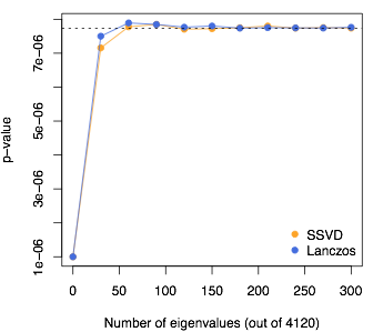
I still need the hundred or so largest eigenvalues. There are at least two ways to get these with much less effort than a full eigendecomposition: Lanczos-type algorithms and stochastic Singular Value Decomposition. They both work, about equally fast and about equally accurately, to reduce the time complexity from \(n^3\) to \(n^2k\) for \(k\) largest eigenvalues.
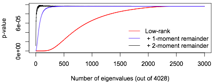
This isn’t just a low-rank approximation: the \(a_k\chi^2_{\nu_k}\) term is important. If we took a low-rank approximation to \(A\) with no remainder term, we would need to take \(k\) large enough that the sum of first \(k\) eigenvalues was close to the sum of all the eigenvalues. The leading-eigenvalue approximation is much better. Here’s an example comparing them, where I cheat (but also make things more comparable) by working out the full eigendecomposition first. Using just the first \(k\) eigenvalues in a low-rank approximation to \(A\) we need \(k>2000\), but using the first \(k\) eigenvalues plus a remainder term we only need about \(k=50\). A low-rank approximation needs \(k\approx 350\) to do even as well as the leading-eigenvalue approximation with \(k=0\)!
In fact, you can do pretty well even using a remainder term that gets only the mean right: replace the remainder term by \(b_k\chi^2_{n-k}\) with \[b_k=\frac{1}{n-k}\sum_{j=k+1}^n\lambda_i.\]
In this graph the red line shows what happens (for a single example) using no remainder term, the blue line uses the remainder term with the right mean, and the black line uses the proposed remainder term with the right mean and variance.
What’s more, in the genomic setting, \(A\) is a weighted covariance for a \(m\times n\) sparse genotype matrix. While \(A\) isn’t sparse and doesn’t have a sparse square root, it can be written as the product of a sparse matrix and a projection matrix of low rank, so that multiplication by \(A\) can be done fast. A ‘matrix-free’ version of the algorithm, which uses \(A\) only via matrix-vector multiplications, has a time complexity of something like \(O(\alpha mnk+np^2k)\) where \(\alpha\) is the fraction of non-zero elements in the matrix of genotypes (typically only a few percent) and \(p\) is the number of adjustment variables in the model.
For 5000 (simulated) individuals and 20,000 variants the sparse version of the new approximation is 3.5 orders of magnitude faster than using a full eigendecomposition. More importantly, taking advantage of sparse genotypes makes it possible to look at really large classes of potentially-functional variants that wouldn’t otherwise be feasible – classes defined by epigenetic markers or by structural features of the chromosome.
Software here. ASHG abstract here.