Variation explained and log transformation

This post is technical details for one at StatsChat on the Johns Hopkins “two-thirds of cancer is bad luck” paper.

I don’t have any real opinions on the conclusion: it’s clear that unforced errors  in DNA copying will cause some cancers, and it’s not obvious how many.  The technical problem with the paper (or at least with its publicity) is that the ‘proportion of variation explained’ was estimated for log risk and quoted as “two-thirds of cancers are due to bad luck’.

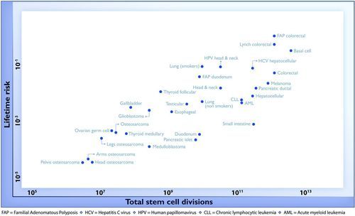
This is the graph, with the impressive linear relationship, 

 

I downloaded the supplementary material and extracted the data from the (ugh) multi-page PDF table (thanks, Tabula), and I agree with the researchers

> with(vogel, cor(log(incidence),log(divcum)))
[1] 0.8039453 

The proportion of variation explained in that graph is \(0.804^2=0.65\), but the y-axis variable in that graph isn’t cancer risk. It’s log cancer risk.  As you can see visually, the log transformation makes the variation about the same in rare cancers as common ones. However, from a population point of view, a two-fold variation in a common cancer is much more important than a two-fold variation in a rare cancer.

There are at least two ways around this.  The first is to work out the implied power-curve model for risk.  The slope in the log-log plot is very close to 0.5, so this suggests looking at the correlation between incidence and square root of stem cell divisions

> with(vogel, cor(incidence,sqrt(divcum)))
[1] 0.5968341
> with(vogel, cor(incidence,sqrt(divcum)))^2
[1] 0.3562109

That’s what I did on StatsChat.  I also searched a bit to see if you could do better than a square root transformation, but without success.

The other thing you could do is a weighted analysis.  From the delta method, we can see that the variance of \(\log(\textrm{incidence})\) is the variance of \(\textrm{incidence}\) divided by \(\textrm{incidence}^2\).  If we weight the residuals by incidence, we approximately cancel out the effect of the transformation and get a proportion of incidence explained.

> summary(lm(log(incidence)~log(divcum),data=vogel,weights=incidence))

Call:
lm(formula = log(incidence) ~ log(divcum), data = vogel, weights = incidence)

Weighted Residuals:
     Min       1Q   Median       3Q      Max 
-0.59149 -0.22083 -0.05411 -0.01917  0.69178 

Coefficients:
            Estimate Std. Error t value Pr(>|t|)    
(Intercept) -14.8822     2.9132  -5.108 1.88e-05 ***
log(divcum)   0.5107     0.1063   4.806 4.35e-05 ***
---
Signif. codes:  0 ‘***’ 0.001 ‘**’ 0.01 ‘*’ 0.05 ‘.’ 0.1 ‘ ’ 1

Residual standard error: 0.254 on 29 degrees of freedom
Multiple R-squared:  0.4433,    Adjusted R-squared:  0.4241 

This approach gives 44% rather than 36%, but that’s reasonable agreement for the approximation over such a large range of values. Using cell divisions as the weight gives 0.43.

[On top of this, as I said on StatsChat, the familial colorectal cancers shouldn’t really be in the regression if you are interested in population risk explained.]